Using data augmentation to improve performance with the tf.data and tf.image APIs
Data augmentation is a powerful technique we can apply to artificially increment the size of our dataset, by creating slightly modified copies of the images at our disposal. In this recipe, we'll leverage the tf.data and tf.image APIs to increase the performance of a CNN trained on the challenging Caltech 101 dataset.
Getting ready
We must install tensorflow_docs:
$> pip install git+https://github.com/tensorflow/docs
In this recipe, we'll use the Caltech 101 dataset, which is available here: http://www.vision.caltech.edu/Image_Datasets/Caltech101/. Download and decompress 101_ObjectCategories.tar.gz to your preferred location. From now on, we assume the data is inside the ~/.keras/datasets directory, in a folder named 101_ObjectCategories.
Here are some sample images from Caltech 101:
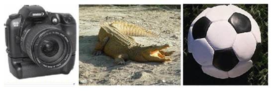
Figure 2.11 – Caltech 101 sample images
Let's go to the next section.
How to do it…
Let's go over the steps required to complete this recipe.
- Import the necessary dependencies:
import os
import pathlib
import matplotlib.pyplot as plt
import numpy as np
import tensorflow as tf
import tensorflow_docs as tfdocs
import tensorflow_docs.plots
from glob import glob
from sklearn.model_selection import train_test_split
from tensorflow.keras.layers import *
from tensorflow.keras.models import Model
- Create an alias for the
tf.data.experimental.AUTOTUNEflag, which we'll use later on:AUTOTUNE = tf.data.experimental.AUTOTUNE
- Define a function to create a smaller version of VGG. Start by creating the input layer and the first block of two convolutions with 32 filters each:
def build_network(width, height, depth, classes):
    input_layer = Input(shape=(width, height, depth))
    x = Conv2D(filters=32,
               kernel_size=(3, 3),
               padding='same')(input_layer)
    x = ReLU()(x)
    x = BatchNormalization(axis=-1)(x)
    x = Conv2D(filters=32,
               kernel_size=(3, 3),
               padding='same')(x)
    x = ReLU()(x)
    x = BatchNormalization(axis=-1)(x)
    x = MaxPooling2D(pool_size=(2, 2))(x)
    x = Dropout(rate=0.25)(x)
- Continue with the second block of two convolutions, this time each with 64 kernels:
    x = Conv2D(filters=64,
               kernel_size=(3, 3),
               padding='same')(x)
    x = ReLU()(x)
    x = BatchNormalization(axis=-1)(x)
    x = Conv2D(filters=64,
               kernel_size=(3, 3),
               padding='same')(x)
    x = ReLU()(x)
    x = BatchNormalization(axis=-1)(x)
    x = MaxPooling2D(pool_size=(2, 2))(x)
    x = Dropout(rate=0.25)(x)
- Define the last part of the architecture, which consists of a series of fully connected layers:
    x = Flatten()(x)
    x = Dense(units=512)(x)
    x = ReLU()(x)
    x = BatchNormalization(axis=-1)(x)
    x = Dropout(rate=0.5)(x)
    x = Dense(units=classes)(x)
    output = Softmax()(x)
    return Model(input_layer, output)
- Define a function to plot and save the training curves of a model, given its training history:
def plot_model_history(model_history, metric, plot_name): plt.style.use('seaborn-darkgrid') plotter = tfdocs.plots.HistoryPlotter() plotter.plot({'Model': model_history}, metric=metric) plt.title(f'{metric.upper()}') plt.ylim([0, 1]) plt.savefig(f'{plot_name}.png') plt.close() - Define a function to load an image and one-hot encode its label, based on the image's file path:
def load_image_and_label(image_path, target_size=(64,
                                                 64)):
    image = tf.io.read_file(image_path)
    image = tf.image.decode_jpeg(image, channels=3)
    image = tf.image.convert_image_dtype(image,
                                         np.float32)
    image = tf.image.resize(image, target_size)
    label = tf.strings.split(image_path, os.path.sep)[-2]
    label = (label == CLASSES)  # One-hot encode.
    label = tf.dtypes.cast(label, tf.float32)
    return image, label
- Define a function to augment an image by performing random transformations on it:
def augment(image, label):
    image = tf.image.resize_with_crop_or_pad(image,
                                             74, 74)
    image = tf.image.random_crop(image, size=(64, 64, 3))
    image = tf.image.random_flip_left_right(image)
    image = tf.image.random_brightness(image, 0.2)
    return image, label
- Define a function to prepare a
tf.data.Datasetof images, based on a glob-like pattern that refers to the folder where they live:def prepare_dataset(data_pattern): return (tf.data.Dataset .from_tensor_slices(data_pattern) .map(load_image_and_label, num_parallel_calls=AUTOTUNE))
- Set the random seed:
SEED = 999
np.random.seed(SEED)
- Load the paths to all images in the dataset, excepting the ones of the
BACKGROUND_Googleclass:base_path = (pathlib.Path.home() / '.keras' / 'datasets' / '101_ObjectCategories') images_pattern = str(base_path / '*' / '*.jpg') image_paths = [*glob(images_pattern)] image_paths = [p for p in image_paths if p.split(os.path.sep)[-2] != 'BACKGROUND_Google']
- Compute the unique categories in the dataset:
CLASSES = np.unique([p.split(os.path.sep)[-2]
                     for p in image_paths])
- Split the image paths into training and testing subsets:
train_paths, test_paths = train_test_split(image_paths,
                                          test_size=0.2,
                                      random_state=SEED)
- Prepare the training and testing datasets, without augmentation:
BATCH_SIZE = 64
BUFFER_SIZE = 1024
train_dataset = (prepare_dataset(train_paths)
                 .batch(BATCH_SIZE)
                 .shuffle(buffer_size=BUFFER_SIZE)
                 .prefetch(buffer_size=BUFFER_SIZE))
test_dataset = (prepare_dataset(test_paths)
                .batch(BATCH_SIZE)
                .prefetch(buffer_size=BUFFER_SIZE))
- Instantiate, compile, train and evaluate the network:
EPOCHS = 40
model = build_network(64, 64, 3, len(CLASSES))
model.compile(loss='categorical_crossentropy',
              optimizer='rmsprop',
              metrics=['accuracy'])
history = model.fit(train_dataset,
                    validation_data=test_dataset,
                    epochs=EPOCHS)
result = model.evaluate(test_dataset)
print(f'Test accuracy: {result[1]}')
plot_model_history(history, 'accuracy', 'normal')
The accuracy on the test set is:
Test accuracy: 0.6532258
And here's the accuracy curve:

Figure 2.12 – Training and validation accuracy for a network without data augmentation
- Prepare the training and testing sets, this time applying data augmentation to the training set:
train_dataset = (prepare_dataset(train_paths)
                 .map(augment,
                     num_parallel_calls=AUTOTUNE)
                 .batch(BATCH_SIZE)
                 .shuffle(buffer_size=BUFFER_SIZE)
                 .prefetch(buffer_size=BUFFER_SIZE))
test_dataset = (prepare_dataset(test_paths)
                .batch(BATCH_SIZE)
                .prefetch(buffer_size=BUFFER_SIZE))
- Instantiate, compile, train, and evaluate the network on the augmented data:
model = build_network(64, 64, 3, len(CLASSES))
model.compile(loss='categorical_crossentropy',
              optimizer='rmsprop',
              metrics=['accuracy'])
history = model.fit(train_dataset,
                    validation_data=test_dataset,
                    epochs=EPOCHS)
result = model.evaluate(test_dataset)
print(f'Test accuracy: {result[1]}')
plot_model_history(history, 'accuracy', 'augmented')
The accuracy on the test set when we use data augmentation is as follows:
Test accuracy: 0.74711984
And the accuracy curve looks like this:
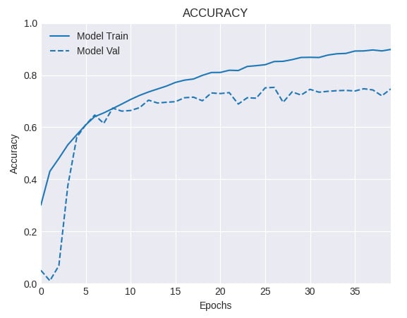
Figure 2.13 – Training and validation accuracy for a network with data augmentation
Let's understand what we just did in the next section.
How it works…
We just implemented a trimmed down version of the famous VGG architecture, trained on the Caltech 101 dataset. To better understand the advantages of data augmentation, we fitted a first version on the original data, without any modification, obtaining an accuracy level of 65.32% on the test set. This first model displays signs of overfitting, because the gap that separates the training and validation accuracy curves widens early in the training process.
Next, we trained the same network on an augmented dataset (see Step 15), using the augment() function defined earlier. This greatly improved the model's performance, reaching a respectable accuracy of 74.19% on the test set. Also, the gap between the training and validation accuracy curves is noticeably smaller, which suggests a regularization effect coming out from the application of data augmentation.
See also
You can learn more about Caltech 101 here: http://www.vision.caltech.edu/Image_Datasets/Caltech101/.


