Scaling with Ray
Ray is a Python native distributed computing framework that was specifically designed to help ML engineers meet the needs of massive data and massively scalable ML systems. Ray has an ethos of making scalable compute available to every ML developer, and in doing this in a way such that you can run anywhere by abstracting out all interactions with underlying infrastructure. One of the unique features of Ray that is particularly interesting is that it has a distributed scheduler, rather than a scheduler or DAG creation mechanism that runs in a central process, like in Spark. At its core, Ray has been developed with compute-intensive tasks such as ML model training in mind from the beginning, which is slightly different from Apache Spark, which has data intensity in mind. You can therefore think about this in a simplified manner: if you need to process lots of data a couple of times, Spark; if you need to process one piece of data lots of times, Ray. This is just a heuristic so should not be followed strictly, but hopefully it gives you a helpful rule of thumb. As an example, if you need to transform millions and millions of rows of data in a large batch process, then it makes sense to use Spark, but if you want to train an ML model on the same data, including hyperparameter tuning, then Ray may make a lot of sense.
The two tools can be used together quite effectively, with Spark transforming the feature set before feeding this into a Ray workload for ML training. This is taken care of in particular by the Ray AI Runtime (AIR), which has a series of different libraries to help scale different pieces of an ML solution. These include:
- Ray Data: Focused on providing data pre-processing and transformation primitives.
- Ray Train: Facilitates large model training.
- Ray Tune: Helps with scalable hyperparameter training.
- Ray RLib: Supports methods for the development of reinforcement learning models.
- Ray Batch Predictor: For batch inference.
- Ray Serving: For re al-time inference.
The AIR framework provides a unified API through which to interact with all of these capabilities and nicely integrates with a huge amount of the standard ML ecosystem that you will be used to, and that we have leveraged in this book.
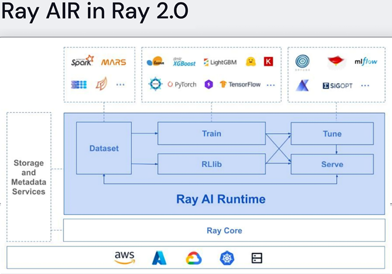
Figure 6.16: The Ray AI runtime, from a presentation by Jules Damji from Anyscale: https://microsites.databricks.com/sites/default/files/2022-07/Scaling%20AI%20Workloads%20with%20the%20Ray%20Ecosystem.pdf. Reproduced with permission.
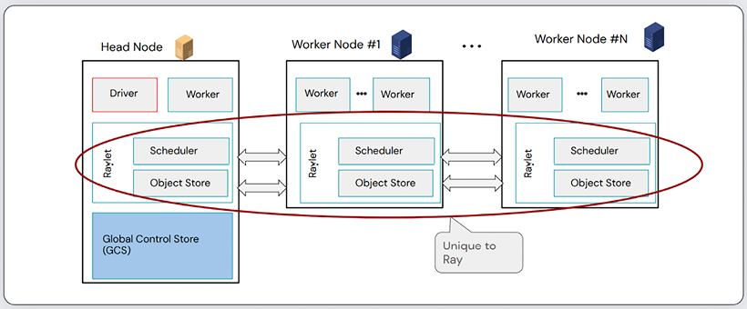
Figure 6.17: The Ray architecture including the Raylet scheduler. From a presentation by Jules Damji: https://microsites.databricks.com/sites/default/files/2022-07/Scaling%20AI%20Workloads%20with%20the%20Ray%20Ecosystem.pdf. Reproduced with permission.
The Ray Core API has a series of different objects that you leverage when using Ray in order to distribute your solution. The first is tasks, which are asynchronous items of work for the system to perform. To define a task, you can take a Python function like:
def add(int: x, int: y) -> int:
    return x+y
And then add the @remote decorator and then use the .remote() syntax in order to submit this task to the cluster. This is not a blocking function so will just return an ID that Ray uses to refer to the task in later computation steps (https://www.youtube.com/live/XME90SGL6Vs?feature=share&t=832) :
import ray

@remote
def add(int: x, int: y) -> int:
    return x+y
add.remote()
In the same vein, the Ray API can extend the same concepts to classes as well; in this case, these are called Actors:
import ray

@ray.remote
class Counter(object):
    def __init__(self):
        self.value = 0
    def increment(self):
        self.value += 1
        return self.value
    def get_counter(self):
        return self.value
# Create an actor from this class.
counter = Counter.remote()
Finally, Ray also has a distributed immutable object store. This is a smart way to have one shared data store across all the nodes of the cluster without shifting lots of data around and using up bandwidth. You can write to the object store with the following syntax:
import ray

numerical_array = np.arange(1,10e7)
obj_numerical_array = ray.put(numerical_array)
new_numerical_array = 0.5*ray.get(obj_numerical_array)
IMPORTANT NOTE
An Actor in this context is a service or stateful worker, a concept used in other distributed frameworks like Akka, which runs on the JVM and has bindings to Java and Scala.
Getting started with Ray for ML
To get started you can install Ray with AI Runtime, as well as some the hyperparameter optimization package, the central dashboard and a Ray enhanced XGBoost implementation, by running:
pip install "ray[air, tune, dashboard]"
pip install xgboost
pip install xgboost_ray
IMPORTANT NOTE
a reminder here that whenver you see pip install in this book, you can also use Poetry as outlined in Chapter 4, Packaging Up. So, in this case, you would have the following commands after running poetry new project_name:
poetry add "ray[air, tune, dashboard]"
poetry add xgboost
poetry add pytorch
Let’s start by looking at Ray Train, which provides an API to a series of Trainer objects that helps facilitate distributed training. At the time of writing, Ray 2.3.0 supports trainers across a variety of different frameworks including:
- Deep learning: Horovod, Tensorflow and PyTorch.
- Tree based: LightGBM and XGBoost.
- Other: Scikit-learn, HuggingFace, and Ray’s reinforcement learning library RLlib.
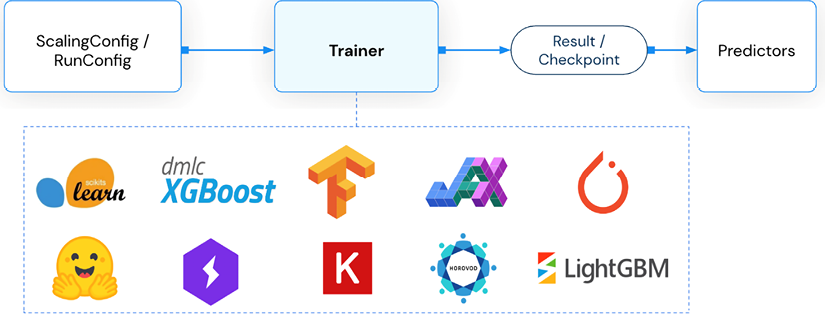
Figure 6.18: Ray Trainers as shown in the Ray docs at https://docs.ray.io/en/latest/train/train.html.
We will first look at a tree-based learner example using XGBoost. Open up a script and begin adding to it; in the repo, this is called getting_started_with_ray.py. What follows is based on an introductory example given in the Ray documentation. First, we can use Ray to download one of the standard datasets; we could also have used sklearn.datasets or another source if we wanted to, like we have done elsewhere in the book:
import ray

dataset = ray.data.read_csv("s3://anonymous@air-example-data/breast_
                             cancer.csv")
train_dataset, valid_dataset = dataset.train_test_split(test_size=0.3)
test_dataset = valid_dataset.drop_columns(cols=["target"])
Note that here we use the ray.data.read_csv() method, which returns a PyArrow dataset. The Ray API has methods for reading from other data formats as well such as JSON or Parquet, as well as from databases like MongoDB or your own custom data sources.
Next, we will define a preprocessing step that will standardize the features we want to use; for more information on feature engineering, you can check out Chapter 3, From Model to Model Factory:
from ray.data.preprocessors import StandardScaler

preprocessor = StandardScaler(columns=["mean radius", "mean texture"])
Then is the fun part where we define the Trainer object for the XGBoost model. This has several different parameters and inputs we will need to define shortly:
from ray.air.config import ScalingConfig
from ray.train.xgboost import XGBoostTrainer

trainer = XGBoostTrainer(
    scaling_config=ScalingConfig(...),
    label_column="target",
    num_boost_round=20,
    params={...},
    datasets={"train": train_dataset, "valid": valid_dataset},
    preprocessor=preprocessor,
)
result = trainer.fit()
You’ll then see something like that shown in Figure 6.19 as output if you run this code in a Jupyter notebook or Python script.
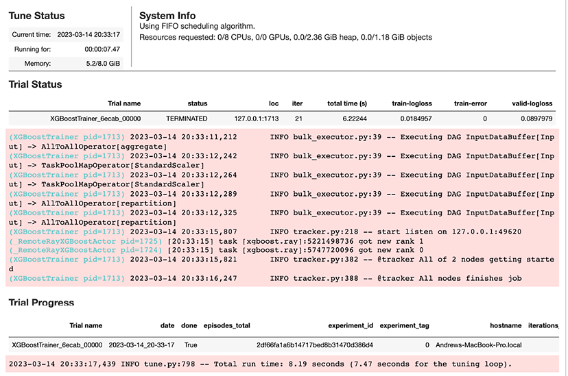
Figure 6.19: Outptut from parallel training of an XGBoost model using Ray.
The result object contains tons of useful information; one of the attributes of it is called metrics and you can print this to reveal details about the end state of the run. Execute print(result.metrics) and you will see something like the following:
{'train-logloss': 0.01849572773292735,
'train-error': 0.0, 'valid-logloss': 0.089797893552767,
'valid-error': 0.04117647058823529,
'time_this_iter_s': 0.019704103469848633,
'should_checkpoint': True,
'done': True,
'timesteps_total': None,
'episodes_total': None,
'training_iteration': 21,
'trial_id': '6ecab_00000',
'experiment_id': '2df66fa1a6b14717bed8b31470d386d4',
'date': '2023-03-14_20-33-17',
'timestamp': 1678825997,
'time_total_s': 6.222438812255859,
'pid': 1713,
'hostname': 'Andrews-MacBook-Pro.local',
'node_ip': '127.0.0.1',
'config': {},
'time_since_restore': 6.222438812255859,
'timesteps_since_restore': 0,
'iterations_since_restore': 21,
'warmup_time': 0.003551006317138672, 'experiment_tag': '0'}
In the instantiation of the XGBoostTrainer, we defined some important scaling information that was omitted in the previous example; here it is:
scaling_config=ScalingConfig(
    num_workers=2,
    use_gpu=False,
    _max_cpu_fraction_per_node=0.9,
)
The num_workers parameter tells Ray how many actors to launch, with each actor by default getting one CPU. The use_gpu flag is set to false since we are not using GPU acceleration here. Finally, by setting the _max_cpu_fraction_per_node parameter to 0.9 we have left some spare capacity on each CPU, which can be used for other operations.
In the previous example, there were also some XGBoost specific parameters we supplied:
params={
    "objective": "binary:logistic",
    "eval_metric": ["logloss", "error"],
}
If you wanted to use GPU acceleration for the XGBoost training you would add tree_method: gpu_hist as a key-value pair in this params dictionary.
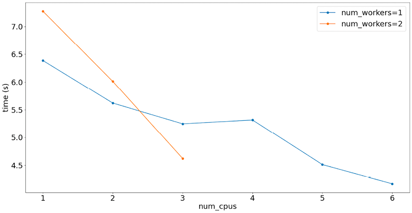
Figure 6.20: A few experiments show how changing the number of workers and CPUs available per worker results in different XGBoost training times on the author’s laptop (an 8 core Macbook Pro).
We will now discuss briefly how you can scale compute with Ray when working in environments other than your local machine.
Scaling your compute for Ray
The examples we’ve seen so far use a local Ray cluster that is automatically set up on the first call to the Ray API. This local cluster grabs all the available CPUs on your machine and makes them available to execute work. Obviously, this will only get you so far. The next stage is to work with clusters that can scale to far larger numbers of available workers in order to get more speedup. You have a few options if you want to do this:
- On the cloud: Ray provides the ability to deploy on to Google Cloud Platform and AWS resources, with Azure deployments handled by a community maintained solution. For more information on deploying and running Ray on AWS, you can check out its online documentation.
- Using Kubernetes: We have already met Kubeflow in Chapter 5, Deployment Patterns and Tools, which is used to build Kubernetes enabled ML pipelines. And we have also discussed Kubernetes in the Containerizing at Scale with Kubernetes section in this chapter.. As mentioned there, Kubernetes is a container orchestration toolkit designed to create massively scalable solutions based on containers. If you want to work with Ray on Kubernetes, you can use the KubeRay project, https://ray-project.github.io/kuberay/.
The setup of Ray on either the cloud or Kubernetes mainly involves defining the cluster configuration and its scaling behaviour. Once you have done this, the beauty of Ray is that scaling your solution is as simple as editing the ScalingConfig object we used in the previous example, and you can keep all your other code the same. So, for example, if you have a 20-node CPU cluster, you could simply change the definition to the following and run it as before:
scaling_config=ScalingConfig(
    num_workers=20,
    use_gpu=False,
    _max_cpu_fraction_per_node=0.9,
)
Scaling your serving layer with Ray
We have discussed the ways you can use Ray to distributed ML training jobs but now let’s have a look at how you can use Ray to help you scale your application layer. As mentioned before, Ray AIR provides some nice functionality for this that is badged under Ray Serve.
Ray Serve is a framework-agnostic library that helps you easily define ML endpoints based on your models. Like with the rest of the Ray API that we have interacted with, it has been built to provide easy interoperability and access to scaling without large development overheads.
Building on the examples from the previous few sections, let us assume we have trained a model, stored it in our appropriate registry, such as MLflow, and we have retrieved this model and have it in memory.
In Ray Serve, we create deployments by using the @ray.serve.deployments decorator. These contain the logic we wish to use to process incoming API requests, including through any ML models we have built. As an example, let’s build a simple wrapper class that uses an XGBoost model like the one we worked with in the previous example to make a prediction based on some pre-processed feature data that comes in via the request object. First, the Ray documentation encourages the use of the Starlette requests library:
from starlette.requests import Request
import ray
from ray import serve
Next we can define the simple class and use the serve decorator to define the service. I will assume that logic for pulling from MLflow or any other model storage location is wrapped into the utility function get_model in the following code block:
@serve.deployment
class Classifier:
    def __init__(self):
        self.model = get_model()
    async def __call__(self, http_request: Request) -> str:
        request_payload = await http_request.json()
        input_vector = [
            request_payload["mean_radius"],
            request_payload["mean_texture"]
        ]
        classification = self.model.predict([input_vector])[0]
        return {"result": classification}
You can then deploy this across an existing Ray cluster.
This concludes our introduction to Ray. We will now finish with a final discussion on designing systems at scale and then a summary of everything we have learned.


