Displaying computation results in Julia

In this recipe, we discuss how to control when Julia displays the results of computations. It is an important part of the standard behavior of Julia code that people often find unclear in their first encounter with the Julia ecosystem. In particular, there are differences in how Julia programs display computation results when running in the console and in script modes, which we explain in this recipe.

Getting ready

Make sure you have the PyPlot package installed by entering using PyPlot in the Julia command line. If it is not installed (an error message will be printed), then run the following command to add it:

julia> using Pkg; Pkg.add("PyPlot")

More details about package management are described in the Managing packages recipe in this chapter.

Then, create the display.jl file in your working directory:

using PyPlot, Random

function f()
    Random.seed!(1)
    r = rand(50)
    @show sum(r)
    display(transpose(r))
    print(transpose(r))
    plot(r)
end

f()

Note

In the GitHub repository for this recipe, you will find the commands.txt file that contains the presented sequence of shell and Julia commands, the display.jl file described above and the display2.jl file described in the recipe.

Now open your favorite terminal to execute the commands.

 

 

How to do it...

In the following steps, we will explain how the output of Julia depends on the context in which a command is invoked:

1. Start the Julia command line and run display.jl in interactive mode:

julia> include("display.jl")
sum(r) = 23.134209483707394
 1×50 LinearAlgebra.Transpose{Float64,Array{Float64,1}}:
 0.236033 0.346517 0.312707 0.00790928 0.488613 0.210968 0.951916 … 0.417039 0.144566 0.622403 0.872334 0.524975 0.241591 0.884837
 [0.236033 0.346517 0.312707 0.00790928 0.488613 0.210968 0.951916 0.999905 0.251662 0.986666 0.555751 0.437108 0.424718 0.773223 0.28119 0.209472 0.251379 0.0203749 0.287702 0.859512 0.0769509 0.640396 0.873544 0.278582 0.751313 0.644883 0.0778264 0.848185 0.0856352 0.553206 0.46335 0.185821 0.111981 0.976312 0.0516146 0.53803 0.455692 0.279395 0.178246 0.548983 0.370971 0.894166 0.648054 0.417039 0.144566 0.622403 0.872334 0.524975 0.241591 0.884837]
 1-element Array{PyCall.PyObject,1}:
 PyObject <matplotlib.lines.Line2D object at 0x0000000026314198>

Apart from the printed value presented earlier, a plot window will open as shown in the following figure:

 

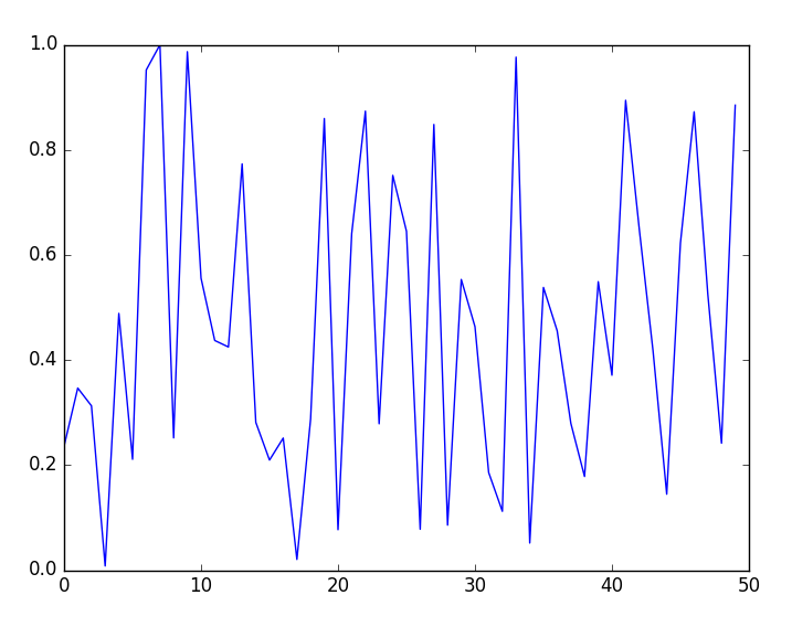
2. Now, exit Julia and run the script in non-interactive mode from the OS shell:

$ julia display.jl
 sum(r) = 23.134209483707394
 1×50 LinearAlgebra.Transpose{Float64,Array{Float64,1}}:
 0.236033 0.346517 0.312707 0.00790928 0.488613 0.210968 0.951916 0.999905 0.251662 0.986666 0.555751 0.437108 0.424718 0.773223 0.28119 0.209472 0.251379 0.0203749 0.287702 0.859512 0.0769509 0.640396 0.873544 0.278582 0.751313 0.644883 0.0778264 0.848185 0.0856352
 0.553206 0.46335 0.185821 0.111981 0.976312 0.0516146 0.53803 0.455692 0.279395 0.178246 0.548983 0.370971 0.894166 0.648054 0.417039 0.144566 0.622403 0.872334 0.524975 0.241591 0.884837[0.236033 0.346517 0.312707 0.00790928 0.488613 0.210968 0.951916 0.999905 0.251662 0.986666 0.555751 0.437108 0.424718 0.773223 0.28119 0.209472 0.251379 0.0203749 0.287702 0.859512 0.0769509 0.640396 0.873544 0.278582 0.751313 0.644883 0.0778264 0.848185 0.0856352 0.553206 0.46335 0.185821 0.111981 0.976312 0.0516146 0.53803 0.455692 0.279395 0.178246 0.548983 0.370971 0.894166 0.648054 0.417039 0.144566 0.622403 0.872334 0.524975 0.241591 0.884837]

In this case, nothing is plotted. Additionally, observe that the display function, in this case, produced a different output than in interactive mode and no newline was inserted after the result (so the output of the print function is visually merged).

3. Now, add show() after plot(r) in the display.jl file and name it display2.jl:

using PyPlot, Random

function f()
    Random.seed!(1)
    r = rand(50)
    @show sum(r)
    display(transpose(r))
    print(transpose(r))
    plot(r)
    show()
end

f()

 

 

4. Run the updated file as a script:

$ julia display2.jl

This time the plot is shown and Julia is suspended until the plot dialog is closed.

How it works...

In Julia, the display function is aware of the context in which it is called. This means that depending on what context is passed to this function, you may obtain a different result. For instance, an image passed to the display in the Julia console usually opens a new window with a plot, but in Jupyter Notebook it might embed it in a notebook. Similarly, many objects in the Julia console are displayed as plain text but in Jupyter Notebook they are converted to a nicely formatted HTML. In short, display(x) typically uses the richest supported multimedia output for x in a given context, with plain text stdout output as a fallback.

In particular, the display function is used by default in the Julia console when a command is executed, for example:

julia> transpose(1:100)
1×100 LinearAlgebra.Transpose{Int64,UnitRange{Int64}}:
 1 2 3 4 5 6 7 8 9 10 11 … 93 94 95 96 97 98 99 100

In this case, the output is adjusted to the size of the Terminal. However, as we saw in the previous example if display is run in a script in non-interactive mode, no adjustment of the output to the size of the device is performed.

An additional issue that is commonly required in practice is suppressing the display of an expression value in the Julia console. This is easily achieved by adding ; at the end of the command, for example:

julia> rand(100, 100);

julia>

And nothing is printed (otherwise, the screen would be flooded by a large matrix).

Finally, in the script in this recipe, we were able to examine the use of the @show macro, which is useful for debugging, as it prints the expression along with its value.

 

 

At the end of this recipe, we observed that the PyPlot package can alter its behavior based on whether it is run in interactive mode or not. Each custom package might have similar specific conditions for handling output to a variety of devices. Being aware of this, it is best to consult the documentation relating to a given package to understand the defaults. If you are developing your own code that needs to be sensitive to the Julia mode (REPL or script) in which it is invoked, there is a handy isinteractive function. This function allows you to dynamically check the Julia interpreter mode at runtime.

There's more...

An in-depth explanation of how display management in Julia works is given at https://docs.julialang.org/en/v1.0/manual/types/#man-custom-pretty-printing-1.

See also

In the Defining your own types - linked list recipe in Chapter 6, Metaprogramming and Advanced Typing, we explain how to specify custom printing for user-defined types.