Search icon CANCEL
Subscription
0
Cart icon
Your Cart (0 item)
Close icon
You have no products in your basket yet
Save more on your purchases! discount-offer-chevron-icon
Savings automatically calculated. No voucher code required.
Arrow left icon
Explore Products
Best Sellers
New Releases
Books
Videos
Audiobooks
Learning Hub
Newsletter Hub
Free Learning
Arrow right icon
timer SALE ENDS IN
0 Days
:
00 Hours
:
00 Minutes
:
00 Seconds
Arrow up icon
GO TO TOP
Python Machine Learning By Example

You're reading from   Python Machine Learning By Example The easiest way to get into machine learning

Arrow left icon
Product type Paperback
Published in May 2017
Publisher Packt
ISBN-13 9781783553112
Length 254 pages
Edition 1st Edition
Languages
Arrow right icon
Authors (2):
Arrow left icon
Yuxi (Hayden) Liu Yuxi (Hayden) Liu
Author Profile Icon Yuxi (Hayden) Liu
Yuxi (Hayden) Liu
Ivan Idris Ivan Idris
Author Profile Icon Ivan Idris
Ivan Idris
Arrow right icon
View More author details
Toc

Table of Contents (9) Chapters Close

Preface 1. Getting Started with Python and Machine Learning FREE CHAPTER 2. Exploring the 20 Newsgroups Dataset with Text Analysis Algorithms 3. Spam Email Detection with Naive Bayes 4. News Topic Classification with Support Vector Machine 5. Click-Through Prediction with Tree-Based Algorithms 6. Click-Through Prediction with Logistic Regression 7. Stock Price Prediction with Regression Algorithms 8. Best Practices

Preprocessing, exploration, and feature engineering

Data mining, a buzzword in the 1990 is the predecessor of data science (the science of data). One of the methodologies popular in the data mining community is called cross industry standard process for data mining (CRISP DM). CRISP DM was created in 1996, and is still used today. I am not endorsing CRISP DM, however I like its general framework. The CRISP DM consists of the following phases, which are not mutually exclusive and can occur in parallel:

  • Business understanding: This phase is often taken care of by specialized domain experts. Usually we have a business person formulate a business problem, such as selling more units of a certain product.
  • Data understanding: This is also a phase, which may require input from domain experts, however, often a technical specialist needs to get involved more than in the business understanding phase. The domain expert may be proficient with spreadsheet programs, but have trouble with complicated data. In this book, I usually call this phase exploration.
  • Data preparation: This is also a phase where a domain expert with only Excel know-how may not be able to help you. This is the phase where we create our training and test datasets. In this book I usually call this phase preprocessing.
  • Modeling: This is the phase, which most people associate with machine learning. In this phase we formulate a model, and fit our data.
  • Evaluation: In this phase, we evaluate our model, and our data to check whether we were able to solve our business problem.
  • Deployment: This phase usually involves setting up the system in a production environment (it is considered good practice to have a separate production system). Typically this is done by a specialized team.

When we learn, we require high quality learning material. We can't learn from gibberish, so we automatically ignore anything that doesn't make sense. A machine learning system isn't able to recognize gibberish, so we need to help it by cleaning the input data. It is often claimed that cleaning the data forms a large part of machine learning. Sometimes cleaning is already done for us, but you shouldn't count on it. To decide how to clean the data, we need to be familiar with the data. There are some projects, which try to automatically explore the data, and do something intelligent, like producing a report. For now, unfortunately, we don't have a solid solution, so you need to do some manual work.

We can do two things, which are not mutually exclusive: first scan the data and second visualize the data. This also depends on the type of data we are dealing with; whether we have a grid of numbers, images, audio, text, or something else. At the end, a grid of numbers is the most convenient form, and we will always work towards having numerical features. I will pretend that we have a table of numbers in the rest of this section.

We want to know if features miss values, how the values are distributed, and what type of features we have. Values can approximately follow a normal distribution, a binomial distribution, a Poisson distribution, or another distribution altogether. Features can be binary: either yes or no, positive or negative, and so on. They can also be categorical: pertaining to a category, for instance continents (Africa, Asia, Europe, Latin America, North America, and so on). Categorical variables can also be ordered—for instance high, medium, and low. Features can also be quantitative, for example temperature in degrees or price in dollars.

Feature engineering is the process of creating or improving features. It's more of a dark art than a science. Features are often created based on common sense, domain knowledge, or prior experience. There are certain common techniques for feature creation, however there is no guarantee that creating new features will improve your results. We are sometimes able to use the clusters found by unsupervised learning as extra features. Deep neural networks are often able to create features automatically.

Missing values

Quite often we miss values for certain features. This could happen for various reasons. It can be inconvenient, expensive, or even impossible to always have a value. Maybe we were not able to measure a certain quantity in the past, because we didn't have the right equipment, or we just didn't know that the feature was relevant. However, we are stuck with missing values from the past. Sometimes it's easy to figure out that we miss values and we can discover this just by scanning the data, or counting the number of values we have for a feature and comparing to the number of values we expect based on the number of rows. Certain systems encode missing values with, for example, values such as 999999. This makes sense if the valid values are much smaller than 999999. If you are lucky, you will have information about the features provided by whoever created the data in the form of a data dictionary or metadata.

Once we know that we miss values the question arises of how to deal with them. The simplest answer is to just ignore them. However, some algorithms can't deal with missing values, and the program will just refuse to continue. In other circumstances, ignoring missing values will lead to inaccurate results. The second solution is to substitute missing values by a fixed value—this is called imputing.

We can impute the arithmetic mean, median or mode of the valid values of a certain feature. Ideally, we will have a relation between features or within a variable that is somewhat reliable. For instance, we may know the seasonal averages of temperature for a certain location and be able to impute guesses for missing temperature values given a date.

Label encoding

Humans are able to deal with various types of values. Machine learning algorithms with some exceptions need numerical values. If we offer a string such as Ivan, unless we are using specialized software the program will not know what to do. In this example, we are dealing with a categorical feature, names probably. We can consider each unique value to be a label. (In this particular example, we also need to decide what to do with the case-is Ivan the same as ivan). We can then replace each label by an integer-label encoding. This approach can be problematic, because the learner may conclude that there is an ordering.

One-hot-encoding

The one-of-K or one-hot-encoding scheme uses dummy variables to encode categorical features. Originally it was applied to digital circuits. The dummy variables have binary values like bits, so they take the values zero or one (equivalent to true or false). For instance, if we want to encode continents, we will have dummy variables, such as is_asia, which will be true if the continent is Asia and false otherwise. In general, we need as many dummy variables, as there are unique labels minus one. We can determine one of the labels automatically from the dummy variables, because the dummy variables are exclusive. If the dummy variables all have a false value, then the correct label is the label for which we don't have a dummy variable. The following table illustrates the encoding for continents:

Is_africa

Is_asia

Is_europe

Is_south_america

Is_north_america

Africa

True

False

False

False

False

Asia

False

True

False

False

False

Europe

False

False

True

False

False

South America

False

False

False

True

False

North America

False

False

False

False

True

Other

False

False

False

False

False

The encoding produces a matrix (grid of numbers) with lots of zeroes (false values) and occasional ones (true values). This type of matrix is called a sparse matrix. The sparse matrix representation is handled well by the SciPy package, and shouldn't be an issue. We will discuss the SciPy package later in this chapter.

Scaling

Values of different features can differ by orders of magnitude. Sometimes this may mean that the larger values dominate the smaller values. This depends on the algorithm we are using. For certain algorithms to work properly we are required to scale the data. There are several common strategies that we can apply:

  • Standardization removes the mean of a feature and divides by the standard deviation. If the feature values are normally distributed, we will get a Gaussian, which is centered around zero with a variance of one.
  • If the feature values are not normally distributed, we can remove the median and divide by the interquartile range. The interquartile range is a range between the first and third quartile (or 25th and 75th percentile).
  • Scaling features to a range is a common choice of range which is a range between zero and one.

Polynomial features

If we have two features a and b, we can suspect that there is a polynomial relation, such as a2 + ab + b2. We can consider each term in the sum to be a feature, in this example we have three features. The product ab in the middle is called an interaction. An interaction doesn't have to be a product, although this is the most common choice, it can also be a sum, a difference or a ratio. If we are using a ratio to avoid dividing by zero, we should add a small constant to the divisor and dividend. The number of features and the order of the polynomial for a polynomial relation are not limited. However, if we follow Occam's razor we should avoid higher order polynomials and interactions of many features. In practice, complex polynomial relations tend to be more difficult to compute and not add much value, but if you really need better results they may be worth considering.

Power transformations

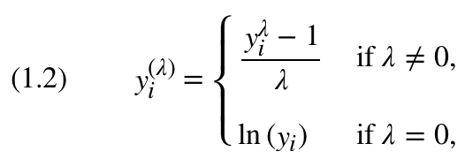
Power transforms are functions that we can use to transform numerical features into a more convenient form, for instance to conform better to a normal distribution. A very common transform for values, which vary by orders of magnitude, is to take the logarithm. Taking the logarithm of a zero and negative values is not defined, so we may need to add a constant to all the values of the related feature before taking the logarithm. We can also take the square root for positive values, square the values, or compute any other power we like.

Another useful transform is the Box-Cox transform named after its creators. The Box-Cox transform attempts to find the best power need to transform the original data into data that is closer to the normal distribution. The transform is defined as follows:

Binning

Sometimes it's useful to separate feature values into several bins. For example, we may be only interested whether it rained on a particular day. Given the precipitation values, we can binarize the values, so that we get a true value if the precipitation value is not zero, and a false value otherwise. We can also use statistics to divide values into high, low, and medium bins.

The binning process inevitably leads to loss of information. However, depending on your goals this may not be an issue, and actually reduce the chance of overfitting. Certainly there will be improvements in speed and memory or storage requirements.

You have been reading a chapter from
Python Machine Learning By Example
Published in: May 2017
Publisher: Packt
ISBN-13: 9781783553112
Register for a free Packt account to unlock a world of extra content!
A free Packt account unlocks extra newsletters, articles, discounted offers, and much more. Start advancing your knowledge today.
Unlock this book and the full library FREE for 7 days
Get unlimited access to 7000+ expert-authored eBooks and videos courses covering every tech area you can think of
Renews at $19.99/month. Cancel anytime
Banner background image