Designing an advanced analytic solution
What are the essential components of an analytic solution? While the exact design can vary between applications, most consist of the following pieces (Figure 1):
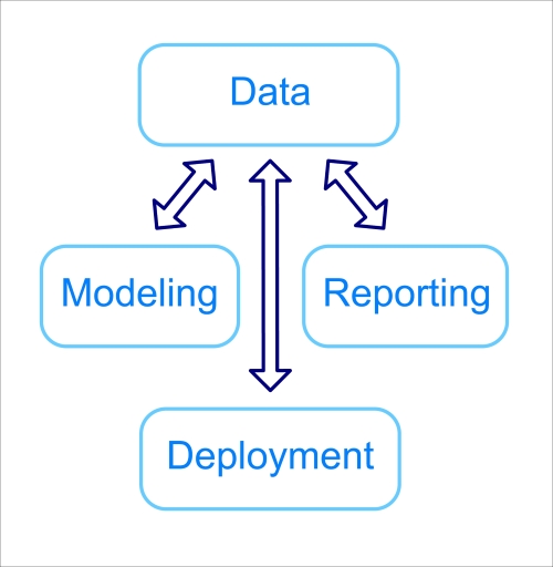
Figure 1: Reference architecture for an analytic pipeline
- Data layer: This stage deals with storage, processing, and persistence of the data, and how it is served to downstream applications such as the analytical applications we will build in this volume. As indicated in Figure 1, data serves as the glue the binds together the other pieces of our application, all of which rely on the data layer to store and update information about their state. This also reflects the separation of concerns that we will discuss in more detail in Chapters 8, Sharing Models with Prediction Services and Chapter 9, Reporting and Testing – Iterating on Analytic Systems, where the other three components of our application can be designed independently since they interact only through the data layer.
- Modeling layer: At this point, the data has been turned into a form that may be ingested by our modeling code in Python. Further feature engineering tasks may be involved to convert this sanitized data into model inputs, along with splitting data into subsets and performing iterative rounds of optimization and tuning. It will also be necessary to prepare the model in a way that can be persisted and deployed to downstream users. This stage is also involved with scoring new data as it is received or performing audits of model health over time.
- Deployment layer: The algorithm development and performance components in the modeling layer are usually exposed to either human users or other software systems through web services, which these consumers interact with through a server layer by means of network calls to both trigger new rounds of model development and query the results of previous analyses.
- Reporting layer: Predictions, model parameters, and insights can all be visualized and automated using reporting services.
With these broad components in mind, let's delve more deeply into the details of each of these pieces.
Data layer: warehouses, lakes, and streams
The beginning of any analytic pipeline is the data itself, which serves as the basis for predictive modeling. This input can vary both in the rate at which updates are available and the amount of transformation that needs to be applied to form the final set of features used in the predictive model. The data layer serves as the repository for this information.
Traditionally, data used for analytics might simply be stored on disk in flat files, such as a spreadsheet or document. As the diversity and scale of data have increased, so have the scale and complexity of resources needed to house and process them. Indeed, a modern view of the data layer encompasses both real-time (stream) data and batch data in the context of many potential downstream uses. This combined system, known as Lambda Architecture (Marz, Nathan, and James Warren. Big Data: Principles and best practices of scalable realtime data systems. Manning Publications Co., 2015.), is diagrammed in the following figure:
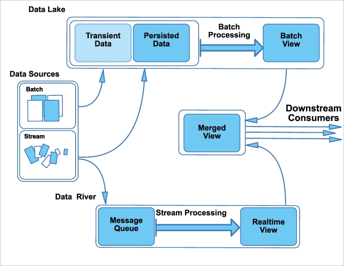
Figure 2: Data layer as a Lambda Architecture
The components of this data layer are:
- Data sources: These could be either real time data received in streams, or batch updates received on a periodic or discontinuous basis.
- Data lake: Both real-time and batch data is commonly saved in a data lake model, in which a distributed file system such as the Hadoop File System (HDFS) or Amazon Web Services (AWS) Simple Storage Service (S3) is used as a common storage medium for data received both in batch and in streams. This data can either be stored with a fixed lifetime (transient) or permanent (persisted) retention policy. This data may then be processed in ongoing batch transformations such as Extract, Load, and Transform (ETL) jobs running in frameworks such as MapReduce or Spark. ETL processes might involve cleaning the data, aggregating it into metrics of interest, or reshaping it into a tabular form from raw inputs. This processing forms the batch layer of the Lambda Architecture, where real-time availability is not expected and latency of minutes to days is acceptable in surfacing views of the data for downstream consumption.
- Data river: While the data lake accumulates all types of raw data in a central location, the data river forms an ongoing message queue where real-time data is dispatched to stream processing tasks. This is also termed the speed layer (Marz, Nathan, and James Warren. Big Data: Principles and best practices of scalable realtime data systems. Manning Publications Co., 2015.) of the architecture, as it operates on data as soon as it is available and real-time availability is expected.
- Merged view: Both real-time and batch views of the raw data may be merged into a common persistence layer, such as a data warehouse in structured tables, where they can be queried using Structured Query Language (SQL) and utilized in either transactional (for example, updating a bank balance in real time) or analytic (for example, running analyses or reports) applications. Examples of such warehouse systems include traditional relational systems such as MySQL and PostgreSQL (which usually store data with tabular schema in rows and columns), and NoSQL systems such as MongoDB or Redis (which arrange data more flexibly in key-value systems, where values can take on numerous formats outside the traditional rows and columns). This merged system is also referred to as the serving layer (Marz, Nathan, and James Warren. Big Data: Principles and best practices of scalable realtime data systems. Manning Publications Co., 2015.), and can either be directly queried using the database system, or surfaced to downstream applications.
- Downstream applications: Systems such as our advanced analytic pipelines can either directly consume the outputs of the batch and real-time processing layers, or interact with one or both of these sources through the merged view in the warehousing system.
How might streaming and batch data be processed differently in the data layer? In batch pipelines, the allowed delay between receiving and processing the data allows for potentially complex transformations of the source data: elements may be aggregated (such as calculating a user or product's average properties over a period of time), joined to other sources (for example, indexing additional website metadata on search logs), and filtered (for example, many web logging systems need to remove bot activity that would otherwise skew the results of predictive models). The source data could be obtained, for example, from simple text files posted to a server, a relational database system, or a mixture of different storage formats (see as follows).
Conversely, due to the speed at which incoming data must often be consumed, streaming processes typically involve less complex processing of inputs than batch jobs, and instead use simple filters or transformations. The sources for such applications are typically continuously updated streams from web services (such as social media or news feeds), events (such as geo-locations of vehicles and mobile phones), or customer activities (such as searches or clicks).
The choice between batch and stream processing at this stage is largely determined by the data source, which is either available as a continuously updated series of events (streaming) or larger, periodically available chunks (batch). In some cases, the nature of the data will also determine the form of the subsequent pipeline and an emphasis on real-time or higher latency processing. In others, the use of the application will take precedent in downstream choices. The normalized view surfaced in the data layer is used downstream in the next stage of the analytic pipeline, the modeling layer.
Modeling layer
The modeling layer involves a number of interconnected tasks, diagrammed in the following figure (Figure 3). As the data layer accommodates both real-time and batch data, we can imagine two main kinds of modeling systems:
- Streaming pipelines act upon a continuous source of data (such as instant messages or a news feed) as soon as it becomes available, potentially allowing real-time model updates or scoring. However, the ability to update the model in real time may vary by algorithm (for example it will work for models using stochastic updates, described in Chapter 5, Putting Data in its Place – Classification Methods and Analysis), and some can only be developed in an offline process. The potential volume of streaming data may also mean that it cannot be stored in its raw form, but only transformed into a more manageable format before the original record is discarded.
- Batch processing. Data sources that are updated on a periodic basis (often daily) are frequently processed using a batch-oriented framework. The input does not need to be used at the moment it is available, with a latency of hours or days between updates usually acceptable, meaning the data processing and model development are typically not occurring in real time.
Note
On the surface, the choice between the two classes of pipelines seems to involve the tradeoff between real-time (streaming) or offline (batch) analysis. In practice, the two classes can have real-time and non-real-time components intermingled within a single application.
If both types of pipeline are viable for a given problem (for example, if the streams are stock prices, a dataset whose volume and simple format – a set of numbers – should allow it to be readily stored offline and processed in its entirety at a later date), the choice between the two frameworks may be dictated by technical or business concerns. For example, sometimes the method used in a predictive model allows only for batch updates, meaning that continuously processing a stream as it is received does not add additional value. In other cases, the importance of the business decisions informed by the predictive model necessitates real-time updates and so would benefit from stream processing.
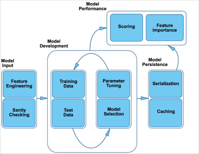
Figure 3: Overview of the modeling layer
The details of the generic components of each type of pipeline as shown in Figure 3 are as follows:
In the Model Input step the source data is loaded and potentially transformed by the pipeline into the inputs required for a predictive model. This can be as simple as exposing a subset of columns in a database table, or transforming an unstructured source such as text into a form that may be input to a predictive model. If we are fortunate, the kinds of features we wish to use in a model are already the form in which they are present in the raw data. In this case, the model fitting proceeds directly on the inputs. More often, the input data just contains the base information we might want to use as inputs to our model, but needs to be processed into a form that can be utilized in prediction.
In the case of numerical data, this might take the form of discretization or transformation. Discretization involves taking a continuous number (such as consumer tenure on a subscription service) and dividing it into bins (such as users with <30 or >=30 days of subscription) that either reduce the variation in the dataset (by thresholding an outlier on a continuous scale to a reasonable bin number) or turn a numerical range into a set of values that have more direct business implications. Another example of discretization is turning a continuous value into a rank, in cases where we don't care as much about the actual number as its relative value compared to others. Similarly, values that vary over exponential scales might be transformed using a natural logarithm to reduce the influence of large values on the modeling process.
In addition to these sorts of transformations, numerical features might be combined in ratios, sums, products, or other combinations, yielding a potential combinatorial explosion of features from even a few basic inputs. In some models, these sorts of interactions need to be explicitly represented by generating such combined features between inputs (such as the regression models we discuss in Chapter 4, Connecting the Dots with Models – Regression Methods). Other models have some ability to decipher these interactions in datasets without our direct creation of the feature (such as random forest algorithms in Chapter 5, Putting Data in its Place – Classification Methods and Analysis or gradient boosted decision trees in Chapter 6, Words and Pixels – Working with Unstructured Data).
In the case of categorical data, such as country codes or days of the week, we may need to transform the category into a numerical descriptor. This could be a number (if the data is ordinal, meaning for example that a value of 2 has an interpretation of being larger than another record with value 1 for that feature) or a vector with one or more non-zero entries indicating the class to which a categorical feature belongs (for example, a document could be represented by a vector the same length as the English vocabulary, with a number indicating how many times each word represented by a particular vector position appears in the document).
Finally, we might find cases where we wish to discover the hidden features represented by a particular set of inputs. For example, income, occupation, and age might all be correlated with the zip code in which a customer lives. If geographic variables aren't part of our dataset, we could still discover these common underlying patterns using dimensionality reduction, as we will discuss in Chapter 6, Words and Pixels – Working with Unstructured Data.
Sanity checking may also be performed at this stage, as it is crucial to spot data anomalies when they appear, such as outliers that might degrade the performance of the model. In the first phase of quality checks, the input data is evaluated to prevent outliers or incorrect data from impacting the quality of models in the following stages. These sanity checks could take many forms: for categorical data (for example, a state or country), there are only a fixed number of allowable values, making it easy to rule out incorrect inputs. In other cases, this quality check is based on an empirical distribution, such as variation from an average value, or a sensible minimum or maximum range. More complex scenarios usually arise from business rules (such as a product being unavailable in a given territory, or a particular combination of IP addresses in web sessions being illogical).
Such quality checks serve as more than safeguards for the modeling process: they can also serve as warnings of events such as bot traffic on websites that may indicate malicious activity. Consequently, these audit rules may also be incorporated as part of the visualization and reporting layer at the conclusion of the pipeline.
In the second round of quality checks following model development, we want to evaluate whether the parameters of the model make sense and whether the performance on the test data is in an acceptable range for deployment. The former might involve plotting the important parameters of a model if the technique permits, visualizations that can then also be utilized by the reporting step downstream. Similarly, the second class of checks can involve looking at accuracy statistics such as precision, recall, or squared error, or the similarity of the test set to data used in model generation in order to determine if the reported performance is reasonable.
As with the first round of sanity checks, not only can these quality control measures serve to monitor the health of the model development process, but also potentially highlight changes in the actual modeling code itself (especially if this code is expected to be regularly updated).
There isn't inherently much difference between streaming and batch-oriented processing in the sanity checking process, just the latency at which the application can uncover anomalies in the source data or modelling process and deliver them to the reporting layer. The complexity of the sanity checks may guide this decision: simple checks that can be done in real-time are well suited for stream processing, while evaluation of the properties of a predictive model could potentially take longer than the training of the algorithm itself, and is thus more suited for a batch process.
In the model development or update step, once the input data has undergone any necessary processing or transformation steps and passed the quality checks described above, it is ready to be used in developing a predictive model. This phase of the analytic pipeline can have several steps, with the exact form depending upon the application:
- Data splitting: At this stage we typically split data into disjoin sets, the training data (from which we will tune the parameters of the algorithm), and the test data (which is used for evaluation purposes). The important reason for making this split is so that the model generalizes to data beyond its initial inputs (the training data), which we can check by evaluating its performance on the test set.
- Parameter tuning: As we will examine in more detail in subsequent chapters, many predictive models have a number of hyperparameters— variables that need to be set before the parameters of the model can be optimized for a training set. Examples include the number of groups in a clustering application (Chapter 3, Finding Patterns in the Noise – Clustering and Unsupervised Learning), the number of trees used in a random forest Chapter 4, Connecting the Dots with Models – Regression Methods, or the learning rate and number of layers in a neural network (Chapter 7, Learning from the Bottom Up – Deep Networks and Unsupervised Features). These hyperparameters frequently need to be calibrated for optimal performance of a predictive model, through grid search (Chapter 5, Putting Data in its Place – Classification Methods and Analysis) or other methods. This tuning can occur only during the initial phase of model development, or as part of a regular retraining cycle. Following or jointly with hyperparameter tuning, the parameters, such as regression coefficients or decision splits in a tree model Chapter 4, Connecting the Dots with Models – Regression Methods, are optimized for a given set of training data. Depending upon the method, this step may also involve variable selection—the process of pruning uninformative features from the input data. Finally, we may perform the above tasks for multiple algorithms and choose the best performing technique.
Batch-oriented and streaming processes could differ at this stage depending upon the algorithm. For example, in models that allow for incremental updates through stochastic learning (Chapter 5, Putting Data in its Place – Classification Methods and Analysis), new data may be processed in a stream as each new training example can individually tune the model parameters. Conversely, data may arrive in a stream but be aggregated until a sufficient size is reached, at which point a batch process is launched to retrain the model. Some models allow for both kinds of training, and the choice depends more on the expected volatility of the input data. For example, rapidly trending signals in social media posts may suggest updating a model as soon as events are available, while models based on longer-term events such as household buying patterns may not justify such continuous updates.
- Model performance: Using either the test data split off during model development or an entirely new set of observations, the modeling layer is also responsible for scoring new data, surfacing important features in the model, and providing information about its ongoing performance. Once the model has been trained on a set of input data, it can be applied to new data in either in real-time computations, or through offline, batch processing to generate a predicted outcome or behavior.
Depending upon the extent of initial data processing, new records may also need to be transformed to generate the appropriate features for evaluation by a model. The extent of such transformations may dictate whether scoring is best accomplished through a streaming or batch framework.
Similarly, the use of the resulting prediction may guide the choice between streaming or batch-oriented processing. When such scores are used as inputs to other, responsive systems (such as in reordering search results or ads presented on a webpage), real-time updates from streaming pipelines, allow for immediate use of the new scores and so may be valuable. When the scores are primarily used for internal decision-making (such as prioritizing sales leads for follow-up), real-time updates may not be necessary and a batch-oriented framework can be used instead. This difference in latency may be correlated with whether the downstream consumer is another application (machine to machine interaction), or a human user relying upon the model for insight (machine to human).
- Model persistence: Once we have tuned the parameters of the predictive model, the result may also need to be packaged, or serialized into a format to allow deployment within a production environment. We will examine this in greater depth in Chapter 8, Sharing Models with Prediction Services, but in brief this process involves transforming the model output into a form for use by downstream systems and saving it back to the data layer for both disaster recovery and potential use by the reporting layer downstream described as follows.
Deployment layer
The output of our predictive modeling can be made broadly available to both individual users and other software services through a deployment layer, which encapsulates the modeling, scoring, and evaluation functions in the previous layer inside of web applications, as shown in the following Figure 4:
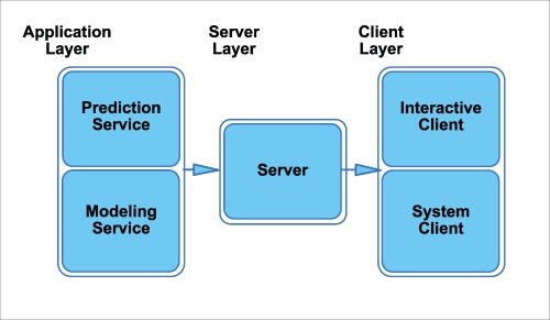
Figure 4: Deployment layer components
This application layer receives network calls over the web, transmitted either through a web browser or from a programmatic request generated by another software system. As we will describe in Chapter 8, Sharing Models with Prediction Services, these applications usually provide a standard set of commands to initiate an action, get a result, save new information, or delete unwanted information. They also typically interact with the data layer to both store results and, in the case of long-running tasks, to store information about the progress of modeling computations.
The network calls received by these applications are brokered by the Server Layer, which serves to route traffic between applications (usually based on url patterns). As we will cover in Chapter 8, Sharing Models with Prediction Services, this separation between the server and application allows us to scale our application by adding more machines, and independently add more servers to balance incoming requests.
The client layer, which initiates the requests received by the server, could be both interactive systems, such as a dashboard, or an independent system such as an e-mail server, that uses the output of a model to schedule outgoing messages.
Reporting layer
The output of the analytical pipeline may be surfaced by the reporting layer, which involves a number of distinct tasks, as shown in the following Figure 5:

Figure 5: Reporting applications for prediction services
- Visualizations: This can allow interactive querying of the source data along with model data such as parameters and feature importance. It can also be used to visualize the output of a model, such as the set of recommendations that would be provided to a user on an e-commerce site, or the risk score assigned to a particular bank account. Because it is frequently used in interactive mode, we may also consider aggregating large model inputs into summarized datasets for lower latency during exploratory sessions. Additionally, visualizations can be either an ad hoc process (such as the interactive notebooks we will examine in future chapters), or a fixed series of graphics (such as the dashboards we will construct in Chapter 9, Reporting and Testing – Iterating on Analytic Systems).
- Audit/Healthcheck: The reporting service involves ongoing monitoring of the application. Indeed, an important factor in developing robust analytic pipelines is regular assessment to ensure that the model is performing as expected. Combining outputs from many previous steps, such as quality control checks and scores for new data, a reporting framework visualizes these statistics and compares them to previous values or a gold standard. This sort of reporting can be used both by the analyst, to monitor the application, and as a way to surface insights uncovered by the modeling process to the larger business organization.
- Comparison reports: This might be used as we iterate on model development through the process of experimentation, as we will discuss in Chapter 9, Reporting and Testing – Iterating on Analytic Systems. Because this analysis may involve statistical measurements, the visualizations might be combined with a service in the deployment layer to calculate significance metrics.
The choice of batch versus streaming processes will often determine whether such reports can be provided in real-time, but just because they are available immediately doesn't imply that such frequency is valuable to the user. For example, even if user response rates to an ad campaign can be collected in real-time, decisions about future advertising programs on these results may be constrained by quarterly business planning. In contrast, trending interest in particular search queries might also allow us to quickly tune the results of a recommendation algorithm, and thus this low-latency signal has value. Again, judgment based on the particular use-case is required.
To conclude this introduction, let's examine a pair of hypothetical applications that illustrates many of the components we've described above. Don't worry too much about the exact meaning of all the terminology, which will be expanded upon in following chapters.


