Search icon CANCEL
Arrow left icon
Explore Products
Best Sellers
New Releases
Books
Videos
Audiobooks
Learning Hub
Conferences
Free Learning
Arrow right icon
Arrow up icon
GO TO TOP
Forecasting Time Series Data with Facebook Prophet

You're reading from   Forecasting Time Series Data with Facebook Prophet Build, improve, and optimize time series forecasting models using the advanced forecasting tool

Arrow left icon
Product type Paperback
Published in Mar 2021
Publisher Packt
ISBN-13 9781800568532
Length 270 pages
Edition 1st Edition
Languages
Tools
Arrow right icon
Author (1):
Arrow left icon
Greg Rafferty Greg Rafferty
Author Profile Icon Greg Rafferty
Greg Rafferty
Arrow right icon
View More author details
Toc

Table of Contents (18) Chapters Close

Preface 1. Section 1: Getting Started
2. Chapter 1: The History and Development of Time Series Forecasting FREE CHAPTER 3. Chapter 2: Getting Started with Facebook Prophet 4. Section 2: Seasonality, Tuning, and Advanced Features
5. Chapter 3: Non-Daily Data 6. Chapter 4: Seasonality 7. Chapter 5: Holidays 8. Chapter 6: Growth Modes 9. Chapter 7: Trend Changepoints 10. Chapter 8: Additional Regressors 11. Chapter 9: Outliers and Special Events 12. Chapter 10: Uncertainty Intervals 13. Section 3: Diagnostics and Evaluation
14. Chapter 11: Cross-Validation 15. Chapter 12: Performance Metrics 16. Chapter 13: Productionalizing Prophet 17. Other Books You May Enjoy

ARCH/GARCH

When the variance of a dataset is not constant over time, ARIMA models face problems with modeling it. In economics and finance, in particular, this can be common. In a financial time series, large returns tend to be followed by large returns and small returns tend to be followed by small returns. The former is called high volatility, and the latter low volatility.

Autoregressive Conditional Heteroscedasticity (ARCH) models were developed to solve this problem. Heteroscedasticity is a fancy way of saying that the variance or spread of the data is not constant throughout, with the opposite term being homoscedasticity. The difference is visualized here:
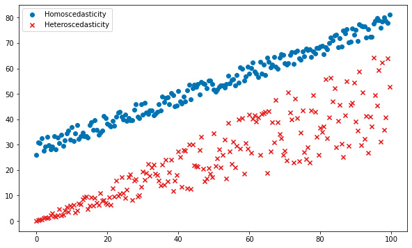
Figure 1.3 – Scedasticity

Figure 1.3 – Scedasticity

Robert Engle introduced the first ARCH model in 1982 by describing the conditional variance as a function of previous values. For example, there is a lot more uncertainty about daytime electricity usage than there is about nighttime usage. In a model of electricity usage, then, we might assume that the daytime hours have a particular variance, and usage during the night would have a lower variance.

Tim Bollerslev and Stephen Taylor introduced a moving average component to the model in 1986 with their Generalized ARCH model, or GARCH. In the electricity example, the variance in usage was a function of time of day. But perhaps the swings in volatility don't necessarily occur at specific times of the day, but the swings are themselves random. This is when GARCH is useful.

Both ARCH and GARCH models can handle neither trend nor seasonality though, so often, in practice, an ARIMA model may first be built to extract out the seasonal variation and trend of a time series, and then an ARCH model may be used to model the expected variance.

You have been reading a chapter from
Forecasting Time Series Data with Facebook Prophet
Published in: Mar 2021
Publisher: Packt
ISBN-13: 9781800568532
Register for a free Packt account to unlock a world of extra content!
A free Packt account unlocks extra newsletters, articles, discounted offers, and much more. Start advancing your knowledge today.
Unlock this book and the full library FREE for 7 days
Get unlimited access to 7000+ expert-authored eBooks and videos courses covering every tech area you can think of
Renews at €18.99/month. Cancel anytime