Gradient Descent

One optimization algorithm that lays the foundation for machine learning models is gradient descent (GD). GD is a simple and effective tool useful to train such models. Gradient descent, as the name suggests, involves “going downhill.” We choose a direction across a landscape and take whichever step gets us downhill. The step size depends on the slope (gradient) of the hill. In machine learning (ML) models, gradient descent estimates the error gradient, helping to minimize the cost function. Very few optimization methods are as computationally efficient as gradient descent. GD also lays the foundation for the optimization of deep learning models.

In problems where the parameters cannot be calculated analytically by use of linear algebra and must be searched by optimization, GD finds its best use. The algorithm works iteratively by moving in the direction of the steepest descent. At each iteration, the model parameters, such as coefficients in linear regression and weights in neural networks, are updated. The model continues to update its parameters until the cost function converges or reaches its minimum value (the bottom of the slope in Figure 4.1a).

Figure 4.1a: Gradient descent

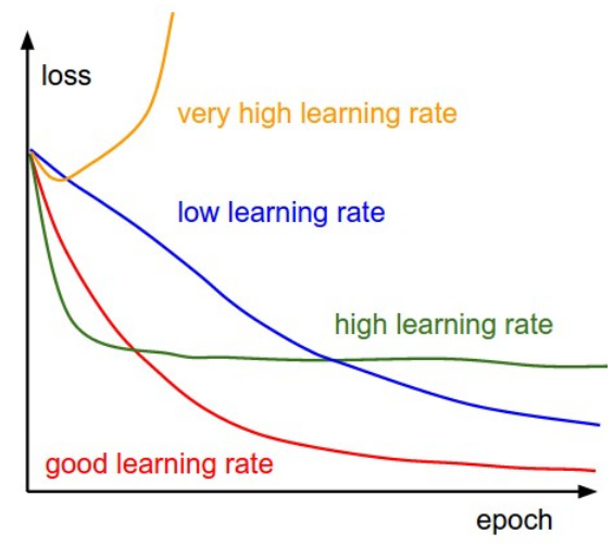
The size of a step taken in each iteration is called the learning rate (a function derivative is scaled by the learning rate at each iteration). With a learning rate that is too low, the model may reach the maximum permissible number of iterations before reaching the bottom, whereas it may not converge or may diverge (the so-called exploding gradient problem) completely if the learning rate is too high. Selecting the most appropriate learning rate is crucial in achieving a model with the best possible accuracy, as seen in Figure 4.1b.

Figure 4.1b: Learning rates in gradient descent

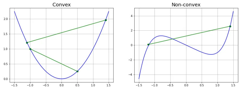
For GD to work, the objective or cost function must be differentiable (meaning the first derivative exists at each point in the domain of a univariate function) and convex (where two points on the function can be connected by a line segment without crossing). The second derivative of a convex function is always positive. Examples of convex and non-convex functions are shown in Figure 4.2. GD is a first-order optimization algorithm.

Figure 4.2: Example of convex (L) and non-convex (R) function

In a multivariate function, the gradient is a vector of derivatives in each direction in the domain. Such functions have saddle points (quasi-convex or semi-convex) where the algorithm may get stuck and obtaining a minimum is not guaranteed. This is where second-order optimization algorithms are brought in to escape the saddle point and reach the global minimum. The GD algorithm finds its use in control as well as mechanical engineering, apart from ML and DL. The following sections compare the algorithm with other optimization algorithms used in ML and deep learning (DL) models and specifically examines some commonly used gradient descent optimizers.

This chapter covers the following topics:

• Gradient descent variants
• Gradient descent optimizers