Search icon CANCEL
Subscription
0
Cart icon
Your Cart (0 item)
Close icon
You have no products in your basket yet
Save more on your purchases! discount-offer-chevron-icon
Savings automatically calculated. No voucher code required.
Arrow left icon
Explore Products
Best Sellers
New Releases
Books
Videos
Audiobooks
Learning Hub
Newsletter Hub
Free Learning
Arrow right icon
timer SALE ENDS IN
0 Days
:
00 Hours
:
00 Minutes
:
00 Seconds
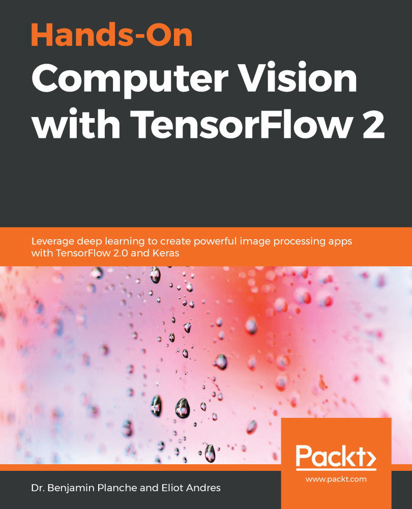
Hands-On Computer Vision with TensorFlow 2

Hands-On Computer Vision with TensorFlow 2: Leverage deep learning to create powerful image processing apps with TensorFlow 2.0 and Keras

Arrow left icon
Profile Icon Benjamin Planche Profile Icon Eliot Andres
Arrow right icon
€8.99 €23.99
Full star icon Full star icon Full star icon Half star icon Empty star icon 3.3 (12 Ratings)
eBook May 2019 372 pages 1st Edition
eBook
€8.99 €23.99
Paperback
€29.99
Subscription
Free Trial
Renews at €18.99p/m
eBook
€8.99 €23.99
Paperback
€29.99
Subscription
Free Trial
Renews at €18.99p/m

What do you get with eBook?

Product feature icon Instant access to your Digital eBook purchase
Product feature icon Download this book in EPUB and PDF formats
Product feature icon Access this title in our online reader with advanced features
Product feature icon DRM FREE - Read whenever, wherever and however you want
Product feature icon AI Assistant (beta) to help accelerate your learning
OR
Modal Close icon
Payment Processing...
tick Completed

Billing Address

Table of content icon View table of contents Preview book icon Preview Book

Hands-On Computer Vision with TensorFlow 2

Computer Vision and Neural Networks

In recent years, computer vision has grown into a key domain for innovation, with more and more applications reshaping businesses and lifestyles. We will start this book with a brief presentation of this field and its history so that we can get some background information. We will then introduce artificial neural networks and explain how they have revolutionized computer vision. Since we believe in learning through practice, by the end of this first chapter, we will even have implemented our own network from scratch!

The following topics will be covered in this chapter:

  • Computer vision and why it is a fascinating contemporary domain
  • How we got there—from local hand-crafted descriptors to deep neural networks
  • Neural networks, what they actually are, and how to implement our own for a basic recognition task
...

Technical requirements

Throughout this book, we will be using Python 3.5 (or higher). As a general-purpose programming language, Python has become the main tool for data scientists thanks to its useful built-in features and renowned libraries.

For this introductory chapter, we will only use two cornerstone libraries—NumPy and Matplotlib. They can be found at and installed from www.numpy.org and matplotlib.org. However, we recommend using Anaconda (www.anaconda.com), a free Python distribution that makes package management and deployment easy.

Complete installation instructions—as well as all the code presented alongside this chapter—can be found in the GitHub repository at github.com/PacktPublishing/Hands-On-Computer-Vision-with-TensorFlow2/tree/master/Chapter01.

We assume that our readers already have some knowledge of Python and a basic understanding of...

Computer vision in the wild

Computer vision is everywhere nowadays, to the point that its definition can drastically vary from one expert to another. In this introductory section, we will paint a global picture of computer vision, highlighting its domains of application and the challenges it faces.

Introducing computer vision

Computer vision can be hard to define because it sits at the junction of several research and development fields, such as computer science (algorithms, data processing, and graphics), physics (optics and sensors), mathematics (calculus and information theory), and biology (visual stimuli and neural processing). At its core, computer vision can be summarized as the automated extraction of information from...

A brief history of computer vision

"Study the past if you would define the future."
– Confucius

In order to better understand the current stand of the heart and current challenges of computer vision, we suggest that we quickly have a look at where it came from and how it has evolved in the past decades.

First steps to initial successes

Scientists have long dreamed of developing artificial intelligence, including visual intelligence. The first advances in computer vision were driven by this idea.

Underestimating the perception task

...

Getting started with neural networks

By now, we know that neural networks form the core of deep learning and are powerful tools for modern computer vision. But what are they exactly? How do they work? In the following section, not only will we tackle the theoretical explanations behind their efficiency, but we will also directly apply this knowledge to the implementation and application of a simple network to a recognition task.

Building a neural network

Artificial neural networks (ANNs), or simply neural networks (NNs), are powerful machine learning tools that are excellent at processing information, recognizing usual patterns or detecting new ones, and approximating complex processes. They have to thank their structure for...

Summary

We covered a lot of ground in this first chapter. We introduced computer vision, the challenges associated with it, and some historical methods, such as SIFT and SVMs. We got familiar with neural networks and saw how they are built, trained, and applied. After implementing our own classifier network from scratch, we can now better understand and appreciate how machine learning frameworks work.

With this knowledge, we are now more than ready to start with TensorFlow in the next chapter.

Questions

  1. Which of the following tasks does not belong to computer vision?
    • A web search for images similar to a query
    • A 3D scene reconstruction from image sequences
    • Animation of a video character
  2. Which activation function were the original perceptrons using?
  3. Suppose we want to train a method to detect whether a handwritten digit is a 4 or not. How should we adapt the network that we implemented in this chapter for this task?

Further reading

TensorFlow 2 and Keras in detail

We have introduced the general architecture of TensorFlow and trained our first model using Keras. Let's now walk through the main concepts of TensorFlow 2. We will explain several core concepts of TensorFlow that feature in this book, followed by some advanced notions. While we may not employ all of them in the remainder of the book, you might find it useful to understand some open source models that are available on GitHub or to get a deeper understanding of the library.

Core concepts

Released in spring 2019, the new version of the framework is focused on simplicity and ease of use. In this section, we will introduce the concepts that TensorFlow relies on and cover how they evolved from version...

The TensorFlow ecosystem

In addition to the main library, TensorFlow offers numerous tools that are useful for machine learning. While some of them are shipped with TensorFlow, others are grouped under TensorFlow Extended (TFX) and TensorFlow Addons. We will now introduce the most commonly used tools.

TensorBoard

While the progress bar we used in the first example of this chapter displayed useful information, we might want to access more detailed graphs. TensorFlow provides a powerful tool for monitoring—TensorBoard. Installed by default with TensorFlow, it is also very easy to use when combined with Keras's callbacks:

callbacks = [tf.keras.callbacks.TensorBoard('./logs_keras')]
model.fit(x_train, y_train, epochs...

Summary

In this chapter, we started by training a basic computer vision model using the Keras API. We introduced the main concepts behind TensorFlow 2—tensors, graphs, AutoGraph, eager execution, and the gradient tape. We also detailed some of the more advanced concepts of the framework. We went through the main tools surrounding the use of deep learning with the library, from TensorBoard for monitoring, to TFX for preprocessing and model analysis. Finally, we covered where to run your model depending on your needs.

With these powerful tools in hand, you are now ready to discover modern computer vision models in the next chapter.

Questions

  1. What is Keras in relation to TensorFlow, and what is its purpose?
  2. Why does TensorFlow use graphs, and how do you create them manually?
  3. What is the difference between eager execution mode and lazy execution mode?
  4. How do you log information in TensorBoard, and how do you display it?
  5. What are the main differences between TensorFlow 1 and TensorFlow 2?

Instance tracking

Some tasks relating video streams could naively be accomplished by studying each frame separately (memory less), but more efficient methods either take into account differences from image to image to guide the process to new frames or take complete image sequences as input for their predictions. Tracking, that is, localizing specific elements in a video stream, is a good example of such a task.

Tracking could be done frame by frame by applying detection and identification methods to each frame. However, it is much more efficient to use previous results to model the motion of the instances in order to partially predict their locations in future frames. Motion continuity is, therefore, a key predicate here, though it does not always hold (such as for fast-moving objects).

Action recognition

On the other hand, action recognition belongs to the list of tasks that can only be run with a sequence of images. Similar to how we cannot understand a sentence when we are given the words separately and unordered, we cannot recognize an action without studying a continuous sequence of images (refer to Figure 1.6).

Recognizing an action means recognizing a particular motion among a predefined set (for instance, for human actions—dancing, swimming, drawing a square, or drawing a circle). Applications range from surveillance (such as the detection of abnormal or suspicious behavior) to human-machine interactions (such as for gesture-controlled devices):

Figure 1.6: Is Barack Obama in the middle of waving, pointing at someone, swatting a mosquito, or something else?
Only the complete sequence of frames could help to label this action
Since object recognition can be split into object classification, detection, segmentation, and so on, so can action recognition...

Motion estimation

Instead of trying to recognize moving elements, some methods focus on estimating the actual velocity/trajectory that is captured in videos. It is also common to evaluate the motion of the camera itself relative to the represented scene (egomotion). This is particularly useful in the entertainment industry, for example, to capture motion in order to apply visual effects or to overlay 3D information in TV streams such as sports broadcasting.

Technical requirements


Throughout this book, we will use TensorFlow 2. You can find detailed installation instructions for the different platforms at: https://www.tensorflow.org/install.

If you plan on using your machine's GPU, make sure you install the corresponding version, tensorflow-gpu. It must be installed along with the CUDA toolkit, a library provided by NVIDIA (https://developer.nvidia.com/cuda-zone).

Installation instructions are also available in the README on GitHub at https://github.com/PacktPublishing/Hands-On-Computer-Vision-with-TensorFlow-2/tree/master/Chapter02.

Getting started with TensorFlow 2 and Keras


Before detailing the core concepts of TensorFlow, we will start with a brief introduction of the framework and a basic example.

Introducing TensorFlow

TensorFlow was originally developed at Google to allow researchers and developers to conduct machine learning research. It was originally defined as an interface for expressing machine learning algorithms, and an implementation for executing such algorithms.

The main promise of TensorFlow is to simplify the deployment of machine learning solutions on various platforms—computer CPU, computer GPUs, mobile devices, and, more recently, in the browser. On top of that, TensorFlow offers many useful functions for creating machine learning models and running them at scale. In 2019, TensorFlow 2 was released with a focus on ease of use while maintaining good performance.

Note

An introduction to TensorFlow 1.0's concepts is available as an Appendix of this book.

The library was open-sourced in November 2015. Since...

TensorFlow 2 and Keras in detail


We introduced the general architecture of TensorFlow and trained our first model using Keras. Let's now walk through the main concepts of TensorFlow 2. We will detail several core concepts of TensorFlow, necessary throughout this book, followed by some advanced notions. While we may not employ all of them in the remainder of the book, the readers might find it useful to understand some open source models available on GitHub or to get a deeper understanding of the library.

Core concepts

Released in spring 2019, the new version of the framework focused on simplicity and ease of use. In this section, we will introduce the concepts that TensorFlow relies on and cover how they evolved from version 1 to version 2.

Introducing tensors

TensorFlow takes its name from a mathematical object called a tensor. You can picture tensors as N-dimensional arrays. A tensor could be a scalar, a vector, a 3D matrix, or an N-dimensional matrix.

A fundamental component of TensorFlow...

TensorFlow ecosystem


On top of the main library, TensorFlow offers numerous tools useful for machine learning. While some of them are shipped with TensorFlow, others are grouped under TensorFlow Extended (TFX) and TensorFlow Addons. We will introduce the most commonly used tools.


TensorBoard

While the progress bar we used in the first example of this chapter displayed useful information, we might want to access more detailed graphs. TensorFlow provides a powerful tool for monitoring—TensorBoard. Installed by default with TensorFlow, it is also very easy to use combined with Keras's callbacks:

callbacks = [tf.keras.callbacks.TensorBoard('./logs_keras')]
model.fit(x_train, y_train, epochs=5, verbose=1, validation_data=(x_test, y_test), callbacks=callbacks)

In this updated code, we pass the TensorBoard callback to the model.fit() method. By default, TensorFlow will automatically write the loss and the metrics to the folder we specified. We can then launch TensorBoard from the command line:

$ tensorboard...

Summary


In this chapter, we started by training a basic computer vision model using the Keras API. We introduced the main concepts behind TensorFlow 2—Tensors, the graph, AutoGraph, eager execution, and the gradient tape. We also detailed some of the more advanced concepts of the framework. We went through the main tools surrounding the use of deep learning with the library, from TensorBoard for monitoring to TFX for pre-processing and model analysis. Finally, we covered where to run your model depending on your needs.

With these powerful tools in hand, you are now ready to discover modern computer vision models in the next chapter.

Questions


  1. What is Keras compared to TensorFlow, and what is its purpose?
  2. Why does TensorFlow use graphs, and how do you create them manually?
  3. What is the difference between eager execution mode and lazy execution mode?
  4. How do you log information in TensorBoard, and how do you display it?
  5. What are the main differences between TensorFlow 1 and TensorFlow 2?

Adding some machine learning on top

It soon appeared clear, however, that extracting robust, discriminative features was only half the job for recognition tasks. For instance, different elements from the same class can look quite different (such as different-looking dogs) and, as a result, share only a small set of common features. Therefore, unlike image-matching tasks, higher-level problems such as semantic classification cannot be solved by simply comparing pixel features from query images with those from labeled pictures (such a procedure can also become sub-optimal in terms of processing time if the comparison has to be done with every image from a large labeled dataset).

This is where machine learning come into play. With an increasing number of researchers trying to tackle image classification in the 90s, more statistical ways to discriminate images based on their features started to appear. Support vector machines (SVMs), which were standardized by Vladimir Vapnik and Corinna...

Rise of deep learning

So, how did neural networks take over computer vision and become what we nowadays know as deep learning? This section offers some answers, detailing the technical development of this powerful tool.

Early attempts and failures

It may be surprising to learn that artificial neural networks appeared even before modern computer vision. Their development is the typical story of an invention too early for its time.

Rise and fall of the perceptron

In the 50s, Frank Rosenblatt came up with the perceptron, a machine learning algorithm inspired by neurons and the underlying block of the first neural networks (The Perceptron: A Probabilistic Model for Information Storage and Organization in the Brain, American Psychological Association, 1958). With the proper learning procedure, this method was already able to recognize characters. However, the hype was short-lived. Marvin Minsky (one of the fathers of AI) and Seymor Papert quickly demonstrated that the perceptron could not learn a function as simple as XOR (exclusive OR, the function that, given two binary input values, returns 1 if one, and only one, input is 1, and returns 0 otherwise). This makes sense to us nowadays—as the perceptron back then was modeled with a linear function while XOR is a non-linear one—but, at that time, it simply discouraged any further research for years.

Too heavy to scale

It was only in the late 70s to early 80s that neural networks got some attention put back on them. Several research papers introduced how neural networks, with multiple layers of perceptrons put one after the other, could be trained using a rather straightforward scheme—backpropagation. As we will detail in the next section, this training procedure works by computing the network's error and backpropagating it through the layers of perceptrons to update their parameters using derivatives. Soon after, the first convolutional neural network (CNN), the ancestor of current recognition methods, was developed and applied to the recognition of handwritten characters with some success.

Alas, these methods were computationally heavy, and just could not scale to larger problems. Instead, researchers adopted lighter machine learning methods such as SVMs, and the use of neural networks stalled for another decade. So, what brought them back and led to the deep learning...

Reasons for the comeback

The reasons for this comeback are twofold and rooted in the explosive evolution of the internet and hardware efficiency.

The internet – the new El Dorado of data science

The internet was not only a revolution in communication; it also deeply transformed data science. It became much easier for scientists to share images and content by uploading them online, leading to the creation of public datasets for experimentation and benchmarking. Moreover, not only researchers but soon everyone, all over the world, started adding new content online, sharing images, videos, and more at an exponential rate. This started big data and the golden age of data science, with the internet as the new El Dorado.

By simply indexing the content that is constantly published online, image and video datasets reached sizes that were never imagined before, from Caltech-101 (10,000 images, published in 2003 by Li Fei-Fei et al., Elsevier) to ImageNet (14+ million images, published in 2009 by Jia Deng et al., IEEE) or Youtube-8M (8+ million videos, published in 2016 by Sami Abu-El-Haija et al., including Google). Even companies...

More power than ever

Luckily, since the internet was booming, so was computing power. Hardware kept becoming cheaper as well as faster, seemingly following Moore's famous law (which states that processor speeds should double every two years—this has been true for almost four decades, though a deceleration is now being observed). As computers got faster, they also became better designed for computer vision. And for this, we have to thank video games.

The graphical processing unit (GPU) is a computer component, that is, a chip specifically designed to handle the kind of operations needed to run 3D games. Therefore, a GPU is optimized to generate or manipulate images, parallelizing these heavy matrix operations. Though the first GPUs were conceived in the 80s, they became affordable and popular only with the advent of the new millennium.

In 2007, NVIDIA, one of the main companies designing GPUs, released the first version of CUDA, a programming language that allows developers...

Deep learning or the rebranding of artificial neural networks

The conditions were finally there for data-hungry, computationally-intensive algorithms to shine. Along with big data and cloud computing, deep learning was suddenly everywhere.

What makes learning deep?

Actually, the term deep learning had already been coined back in the 80s, when neural networks first began stacking two or three layers of neurons. As opposed to the early, simpler solutions, deep learning regroups deeper neural networks, that is, networks with multiple hidden layers—additional layers set between their input and output layers. Each layer processes its inputs and passes the results to the next layer, all trained to extract increasingly abstract information. For instance, the first layer of a neural network would learn to react to basic features in the images, such as edges, lines, or color gradients; the next layer would learn to use these cues to extract more advanced features; and so on until the last layer, which infers the desired output (such as predicted class or detection results).

However, deep learning only really started being used from 2006, when Geoff Hinton and his colleagues proposed an effective solution...

Deep learning era

With research into neural networks once again back on track, deep learning started growing, until a major breakthrough in 2012, which finally gave it its contemporary prominence. Since the publication of ImageNet, a competition (ImageNet Large Scale Visual Recognition Challenge (ILSVRC)—image-net.org/challenges/LSVRC) has been organized every year for researchers to submit their latest classification algorithms and compare their performance on ImageNet with others. The winning solutions in 2010 and 2011 had classification errors of 28% and 26% respectively, and applied traditional concepts such as SIFT features and SVMs. Then came the 2012 edition, and a new team of researchers reduced the recognition error to a staggering 16%, leaving all the other contestants far behind.

In their paper describing this achievement (Imagenet Classification with Deep Convolutional Neural Networks, NIPS, 2012), Alex Krizhevsky, Ilya Sutskever, and Geoff Hinton presented what...

Getting started with neural networks

By now, we know that neural networks form the core of deep learning and are powerful tools for modern computer vision. But what are they exactly? How do they work? In the following section, not only will we tackle the theoretical explanations behind their efficiency, but we will also directly apply this knowledge to the implementation and application of a simple network to a recognition task.

Building a neural network

Artificial neural networks (ANNs), or simply neural networks (NNs), are powerful machine learning tools that are excellent at processing information, recognizing usual patterns or detecting new ones, and approximating complex processes. They have to thank their structure for this, which we will now explore.

Imitating neurons

It is well-known that neurons are the elemental supports of our thoughts and reactions. What might be less evident is how they actually work and how they can be simulated.

Biological inspiration

ANNs are loosely inspired by how animals' brains work. Our brain is a complex network of neurons, each passing information to each other and processing sensory inputs (as electrical and chemical signals) into thoughts and actions. Each neuron receives its electrical inputs from its dendrites, which are cell fibers that propagate the electrical signal from the synapses (the junctions with preceding neurons) to the soma (the neuron's main body). If the accumulated electrical stimulation exceeds a specific threshold, the cell is activated and the electrical impulse is propagated further to the next neurons through the cell's axon (the neuron's output cable, ending with several synapses linking to other neurons). Each neuron can, therefore, be seen as a really simple signal processing unit, which—once stacked together—can achieve the thoughts we are having right now, for instance.

Mathematical model

Inspired by its biological counterpart (represented in Figure 1.11), the artificial neuron takes several inputs (each a number), sums them together, and finally applies an activation function to obtain the output signal, which can be passed to the following neurons in the network (this can be seen as a directed graph):

Figure 1.11: On the left, we can see a simplified biological neuron. On the right, we can see its artificial counterpart

The summation of the inputs is usually done in a weighted way. Each input is scaled up or down, depending on a weight specific to this particular input. These weights are the parameters that are adjusted during the training phase of the network in order for the neuron to react to the correct features. Often, another parameter is also trained and used for this summation process—the neuron's bias. Its value is simply added to the weighted sum as an offset.

Let's quickly formalize this process mathematically. Suppose...

Implementation

Such a model can be implemented really easily in Python (using NumPy for vector and matrix manipulations):

import numpy as np

class Neuron(object):
"""A simple feed-forward artificial neuron.
Args:
num_inputs (int): The input vector size / number of input values.
activation_fn (callable): The activation function.
Attributes:
W (ndarray): The weight values for each input.
b (float): The bias value, added to the weighted sum.
activation_fn (callable): The activation function.
"""
def __init__(self, num_inputs, activation_fn):
super().__init__()
# Randomly initializing the weight vector and bias value:
self.W = np.random.rand(num_inputs)
self.b = np.random.rand(1)
self.activation_fn = activation_fn

def forward(self, x):
"""Forward the input signal through the neuron."""
z = np.dot(x, self.W) + self.b...

Layering neurons together

Usually, neural networks are organized into layers, that is, sets of neurons that typically receive the same input and apply the same operation (for example, by applying the same activation function, though each neuron first sums the inputs with its own specific weights).

Mathematical model

In networks, the information flows from the input layer to the output layer, with one or more hidden layers in-between. In Figure 1.13, the three neurons A, B, and C belong to the input layer, the neuron H belongs to the output or activation layer, and the neurons D, E, F, and G belong to the hidden layer. The first layer has an input, x, of size 2, the second (hidden) layer takes the three activation values of the previous layer as input, and so on. Such layers, with each neuron connected to all the values from the previous layer, are classed as being fully connected or dense:

Figure 1.13: A 3-layer neural network, with two input values and one final output

Once again, we can compact the calculations by representing these elements with vectors and matrices. The following operations are done by the first layers:

This can be expressed as follows:

In order to obtain the previous equation, we must define the variables as follows:

The activation...

Implementation

Like the single neuron, this model can be implemented in Python. Actually, we do not even have to make too many edits compared to our Neuron class:

import numpy as np

class FullyConnectedLayer(object):
"""A simple fully-connected NN layer.
Args:
num_inputs (int): The input vector size/number of input values.
layer_size (int): The output vector size/number of neurons.
activation_fn (callable): The activation function for this layer.
Attributes:
W (ndarray): The weight values for each input.
b (ndarray): The bias value, added to the weighted sum.
size (int): The layer size/number of neurons.
activation_fn (callable): The neurons' activation function.
"""
def __init__(self, num_inputs, layer_size, activation_fn):
super().__init__()
# Randomly initializing the parameters (using a normal distribution this time):
self.W = np.random.standard_normal((num_inputs...

Applying our network to classification

We know how to define layers, but have yet to initialize and connect them into networks for computer vision. To demonstrate how to do this, we will tackle a famous recognition task.

Setting up the task

Classifying images of handwritten digits (that is, recognizing whether an image contains a 0 or a 1 and so on) is a historical problem in computer vision. The Modified National Institute of Standards and Technology (MNIST) dataset (http://yann.lecun.com/exdb/mnist/), which contains 70,000 grayscale images (28 × 28 pixels) of such digits, has been used as a reference over the years so that people can test their methods for this recognition task (Yann LeCun and Corinna Cortes hold all copyrights for this dataset, which is shown in the following diagram):

Figure 1.14: Ten samples of each digit from the MNIST dataset

For digit classification, what we want is a network that takes one of these images as input and returns an output vector expressing how strongly the network believes the image corresponds to each class. The input vector has 28 × 28 = 784 values, while the output has 10 values (for the 10 different digits, from 0 to 9). In-between...

Implementing the network

For the neural network itself, we have to wrap the layers together and add some methods to forward through the complete network and to predict the class according to the output vector. After the layer's implementation, the following code should be self-explanatory:

import numpy as np
from layer import FullyConnectedLayer

def sigmoid(x): # Apply the sigmoid function to the elements of x.
return 1 / (1 + np.exp(-x)) # y

class SimpleNetwork(object):
"""A simple fully-connected NN.
Args:
num_inputs (int): The input vector size / number of input values.
num_outputs (int): The output vector size.
hidden_layers_sizes (list): A list of sizes for each hidden layer to be added to the network
Attributes:
layers (list): The list of layers forming this simple network.
"""

def __init__(self, num_inputs, num_outputs, hidden_layers_sizes=(64, 32)):
super().__init__()
# We build the list...

Training a neural network

Neural networks are a particular kind of algorithm because they need to be trained, that is, their parameters need to be optimized for a specific task by making them learn from available data. Once the networks are optimized to perform well on this training dataset, they can be used on new, similar data to provide satisfying results (if the training was done properly).

Before solving the problem of our MNIST task, we will provide some theoretical background, cover different learning strategies, and present how training is actually done. Then, we will directly apply some of these notions to our example so that our simple network finally learns how to solve the recognition task!

Learning strategies

When it comes to teaching neural networks, there are three main paradigms, depending on the task and the availability of training data.

Supervised learning

Supervised learning may be the most common paradigm, and it is certainly the easiest to grasp. It applies when we want to teach neural networks a mapping between two modalities (for example, mapping images to their class labels or to their semantic masks). It requires access to a training dataset containing both the images and their ground truth labels (such as the class information per image or the semantic masks).

With this, the training is then straightforward:

  • Give the images to the network and collect its results (that is, predicted labels).
  • Evaluate the network's loss, that is, how wrong its predictions are when comparing it to the ground truth labels.
  • Adjust the network parameters accordingly to reduce this loss.
  • Repeat until the network converges, that is, until it cannot improve further on this training data.

Therefore, this strategy deserves the adjective supervised—an entity (us) supervises the training of the network by providing it with...

Unsupervised learning

However, how do we train a network when we do not have any ground truth information available? Unsupervised learning is one answer to this. The idea here is to craft a function that computes the network's loss only based on its input and its corresponding output.

This strategy applies very well to applications such as clustering (grouping images with similar properties together) or compression (reducing the content size while preserving some properties). For clustering, the loss function could measure how similar images from one cluster are compared to images from other clusters. For compression, the loss function could measure how well preserved the important properties are in the compressed data compared to the original ones.

Unsupervised learning thus requires some expertise regarding the use cases so that we can come up with meaningful loss functions.

Reinforcement learning

Reinforcement learning is an interactive strategy. An agent navigates through an environment (for example, a robot moving around a room or a video game character going through a level). The agent has a predefined list of actions it can make (walk, turn, jump, and so on) and, after each action, it ends up in a new state. Some states can bring rewards, which are immediate or delayed, and positive or negative (for instance, a positive reward when the video game character touches a bonus item, and a negative reward when it is hit by an enemy). 

At each instant, the neural network is provided only with observations from the environment (for example, the robot's visual feed, or the video game screen) and reward feedback (the carrot and stick). From this, it has to learn what brings higher rewards and estimate the best short-term or long-term policy for the agent accordingly. In other words, it has to estimate the series of actions that would maximize its...

Teaching time

Whatever the learning strategy, the overall training steps are the same. Given some training data, the network makes its predictions and receives some feedback (such as the results of a loss function), which is then used to update the network's parameters. These steps are then repeated until the network cannot be optimized further. In this section, we will detail and implement this process, from loss computation to weights optimization.

Evaluating the loss

The goal of the loss function is to evaluate how well the network, with its current weights, is performing. More formally, this function expresses the quality of the predictions as a function of the network's parameters (such as its weights and biases). The smaller the loss, the better the parameters are for the chosen task.

Since loss functions represent the goal of networks (return the correct labels, compress the image while preserving the content, and so on), there are as many different functions as there are tasks. Still, some loss functions are more commonly used than others. This is the case for the sum-of-squares function, also called L2 loss (based on the L2 norm), which is omnipresent in supervised learning. This function simply computes the squared difference between each element of the output vector y (the per-class probabilities estimated by our network) and each element of the ground truth vector ytrue (the target vector with null values for every...

Backpropagating the loss

How can we update the network parameters so that they minimize the loss? For each parameter, what we need to know is how slightly changing its value would affect the loss. If we know which changes would slightly decrease the loss, then it is just a matter of applying these changes and repeating the process until reaching a minimum. This is exactly what the gradient of the loss function expresses, and what the gradient descent process is.

At each training iteration, the derivatives of the loss with respect to each parameter of the network are computed. These derivatives indicate which small changes to the parameters need to be applied (with a -1 coefficient since the gradient indicates the direction of increase of the function, while we want to minimize it). It can be seen as walking step by step down the slope of the loss function with respect to each parameter, hence the name gradient descent for this iterative process (refer to the following diagram...

Teaching our network to classify

So far, we have only implemented the feed-forward functionality for our network and its layers. First, let's update our FullyConnectedLayer class so that we can add methods for backpropagation and optimization:

class FullyConnectedLayer(object):
# [...] (code unchanged)
def __init__(self, num_inputs, layer_size, activation_fn, d_activation_fn):
# [...] (code unchanged)
self.d_activation_fn = d_activation_fn # Deriv. activation function
self.x, self.y, self.dL_dW, self.dL_db = 0, 0, 0, 0 # Storage attr.

def forward(self, x):
z = np.dot(x, self.W) + self.b
self.y = self.activation_fn(z)
self.x = x # we store values for back-propagation
return self.y

def backward(self, dL_dy):
"""Back-propagate the loss."""
dy_dz = self.d_activation_fn(self.y) # = f'
dL_dz = (dL_dy * dy_dz) # dL/dz = dL/dy * dy/dz = l'_{k+1} * f'
dz_dw...

Training considerations underfitting and overfitting

We invite you to play around with the framework we just implemented, trying different hyperparameters (layer sizes, learning rate, batch size, and so on). Choosing the proper topography (as well as other hyperparameters) can require lots of tweaking and testing. While the sizes of the input and output layers are conditioned by the use case (for example, for classification, the input size would be the number of pixel values in the images, and the output size would be the number of classes to predict from), the hidden layers should be carefully engineered.

For instance, if the network has too few layers, or the layers are too small, the accuracy may stagnate. This means the network is underfitting, that is, it does not have enough parameters for the complexity of the task. In this case, the only solution is to adopt a new architecture that is more suited to the application.

On the other hand, if the network is too complex...

Summary

We covered a lot of ground in this first chapter. We introduced computer vision, the challenges associated with it, and some historical methods, such as SIFT and SVMs. We got familiar with neural networks and saw how they are built, trained, and applied. After implementing our own classifier network from scratch, we can now better understand and appreciate how machine learning frameworks work.

With this knowledge, we are now more than ready to start with TensorFlow in the next chapter.

Questions

  1. Which of the following tasks does not belong to computer vision?
    • A web search for images similar to a query
    • A 3D scene reconstruction from image sequences
    • Animation of a video character
  2. Which activation function were the original perceptrons using?
  3. Suppose we want to train a method to detect whether a handwritten digit is a 4 or not. How should we adapt the network that we implemented in this chapter for this task?

Further reading

Left arrow icon Right arrow icon
Download code icon Download Code

Key benefits

  • Discover how to build, train, and serve your own deep neural networks with TensorFlow 2 and Keras
  • Apply modern solutions to a wide range of applications such as object detection and video analysis
  • Learn how to run your models on mobile devices and web pages and improve their performance

Description

Computer vision solutions are becoming increasingly common, making their way into fields such as health, automobile, social media, and robotics. This book will help you explore TensorFlow 2, the brand new version of Google's open source framework for machine learning. You will understand how to benefit from using convolutional neural networks (CNNs) for visual tasks. Hands-On Computer Vision with TensorFlow 2 starts with the fundamentals of computer vision and deep learning, teaching you how to build a neural network from scratch. You will discover the features that have made TensorFlow the most widely used AI library, along with its intuitive Keras interface. You'll then move on to building, training, and deploying CNNs efficiently. Complete with concrete code examples, the book demonstrates how to classify images with modern solutions, such as Inception and ResNet, and extract specific content using You Only Look Once (YOLO), Mask R-CNN, and U-Net. You will also build generative adversarial networks (GANs) and variational autoencoders (VAEs) to create and edit images, and long short-term memory networks (LSTMs) to analyze videos. In the process, you will acquire advanced insights into transfer learning, data augmentation, domain adaptation, and mobile and web deployment, among other key concepts. By the end of the book, you will have both the theoretical understanding and practical skills to solve advanced computer vision problems with TensorFlow 2.0.

Who is this book for?

If you’re new to deep learning and have some background in Python programming and image processing, like reading/writing image files and editing pixels, this book is for you. Even if you’re an expert curious about the new TensorFlow 2 features, you’ll find this book useful. While some theoretical concepts require knowledge of algebra and calculus, the book covers concrete examples focused on practical applications such as visual recognition for self-driving cars and smartphone apps.

What you will learn

  • Create your own neural networks from scratch
  • Classify images with modern architectures including Inception and ResNet
  • Detect and segment objects in images with YOLO, Mask R-CNN, and U-Net
  • Tackle problems faced when developing self-driving cars and facial emotion recognition systems
  • Boost your application's performance with transfer learning, GANs, and domain adaptation
  • Use recurrent neural networks (RNNs) for video analysis
  • Optimize and deploy your networks on mobile devices and in the browser

Product Details

Country selected
Publication date, Length, Edition, Language, ISBN-13
Publication date : May 30, 2019
Length: 372 pages
Edition : 1st
Language : English
ISBN-13 : 9781788839266
Category :
Languages :
Tools :

What do you get with eBook?

Product feature icon Instant access to your Digital eBook purchase
Product feature icon Download this book in EPUB and PDF formats
Product feature icon Access this title in our online reader with advanced features
Product feature icon DRM FREE - Read whenever, wherever and however you want
Product feature icon AI Assistant (beta) to help accelerate your learning
OR
Modal Close icon
Payment Processing...
tick Completed

Billing Address

Product Details

Publication date : May 30, 2019
Length: 372 pages
Edition : 1st
Language : English
ISBN-13 : 9781788839266
Category :
Languages :
Tools :

Packt Subscriptions

See our plans and pricing
Modal Close icon
€18.99 billed monthly
Feature tick icon Unlimited access to Packt's library of 7,000+ practical books and videos
Feature tick icon Constantly refreshed with 50+ new titles a month
Feature tick icon Exclusive Early access to books as they're written
Feature tick icon Solve problems while you work with advanced search and reference features
Feature tick icon Offline reading on the mobile app
Feature tick icon Simple pricing, no contract
€189.99 billed annually
Feature tick icon Unlimited access to Packt's library of 7,000+ practical books and videos
Feature tick icon Constantly refreshed with 50+ new titles a month
Feature tick icon Exclusive Early access to books as they're written
Feature tick icon Solve problems while you work with advanced search and reference features
Feature tick icon Offline reading on the mobile app
Feature tick icon Choose a DRM-free eBook or Video every month to keep
Feature tick icon PLUS own as many other DRM-free eBooks or Videos as you like for just €5 each
Feature tick icon Exclusive print discounts
€264.99 billed in 18 months
Feature tick icon Unlimited access to Packt's library of 7,000+ practical books and videos
Feature tick icon Constantly refreshed with 50+ new titles a month
Feature tick icon Exclusive Early access to books as they're written
Feature tick icon Solve problems while you work with advanced search and reference features
Feature tick icon Offline reading on the mobile app
Feature tick icon Choose a DRM-free eBook or Video every month to keep
Feature tick icon PLUS own as many other DRM-free eBooks or Videos as you like for just €5 each
Feature tick icon Exclusive print discounts

Frequently bought together


Stars icon
Total 95.97
Hands-On Computer Vision with TensorFlow 2
€29.99
Hands-On Neural Networks with TensorFlow 2.0
€32.99
Deep Learning with TensorFlow 2 and Keras
€32.99
Total 95.97 Stars icon
Banner background image

Table of Contents

15 Chapters
Section 1: TensorFlow 2 and Deep Learning Applied to Computer Vision Chevron down icon Chevron up icon
Computer Vision and Neural Networks Chevron down icon Chevron up icon
TensorFlow Basics and Training a Model Chevron down icon Chevron up icon
Modern Neural Networks Chevron down icon Chevron up icon
Section 2: State-of-the-Art Solutions for Classic Recognition Problems Chevron down icon Chevron up icon
Influential Classification Tools Chevron down icon Chevron up icon
Influential Classification Tools
Technical requirements
Understanding advanced CNN architectures
VGG – a standard CNN architecture
Overview of the VGG architecture
Motivation
Architecture
Contributions – standardizing CNN architectures
Replacing large convolutions with multiple smaller ones
Increasing the depth of the feature maps
Augmenting data with scale jittering
Replacing fully connected layers with convolutions
Implementations in TensorFlow and Keras
The TensorFlow model
The Keras model
GoogLeNet and the inception module
Overview of the GoogLeNet architecture
Motivation
Architecture
Contributions – popularizing larger blocks and bottlenecks
Capturing various details with inception modules
Using 1 x 1 convolutions as bottlenecks
Pooling instead of fully connecting
Fighting vanishing gradient with intermediary losses
Implementations in TensorFlow and Keras
Inception module with the Keras Functional API
TensorFlow model and TensorFlow Hub
The Keras model
ResNet – the residual network
Overview of the ResNet architecture
Motivation
Architecture
Contributions – forwarding the information more deeply
Estimating a residual function instead of a mapping
Going ultra-deep
Implementations in TensorFlow and Keras
Residual blocks with the Keras Functional API
The TensorFlow model and TensorFlow Hub
The Keras model
Leveraging transfer learning
Overview
Definition
Human inspiration
Motivation
Transferring CNN knowledge
Use cases
Similar tasks with limited training data
Similar tasks with abundant training data
Dissimilar tasks with abundant training data
Dissimilar tasks with limited training data
Transfer learning with TensorFlow and Keras
Model surgery
Removing layers
Grafting layers
Selective training
Restoring pretrained parameters
Freezing layers
Summary
Questions
Further reading
Object Detection Models Chevron down icon Chevron up icon
Enhancing and Segmenting Images Chevron down icon Chevron up icon
Section 3: Advanced Concepts and New Frontiers of Computer Vision Chevron down icon Chevron up icon
Training on Complex and Scarce Datasets Chevron down icon Chevron up icon
Training on Complex and Scarce Datasets
Technical requirements
Efficient data serving
Introducing the TensorFlow Data API
Intuition behind the TensorFlow Data API
Feeding fast and data-hungry models
Inspiration from lazy structures
Structure of TensorFlow data pipelines
Extract, Transform, Load
API interface
Setting up input pipelines
Extracting (from tensors, text files, TFRecord files, and more)
From NumPy and TensorFlow data
From files
From other inputs (generator, SQL database, range, and others)
Transforming the samples (parsing, augmenting, and more)
Parsing images and labels
Parsing TFRecord files
Editing samples
Transforming the datasets (shuffling, zipping, parallelizing, and more)
Structuring datasets
Merging datasets
Loading
Optimizing and monitoring input pipelines
Following best practices for optimization
Parallelizing and prefetching
Fusing operations
Passing options to ensure global properties
Monitoring and reusing datasets
Aggregating performance statistics
Caching and reusing datasets
How to deal with data scarcity
Augmenting datasets
Overview
Why augment datasets?
Considerations
Augmenting images with TensorFlow
TensorFlow Image module
Example – augmenting images for our autonomous driving application
Rendering synthetic datasets
Overview
Rise of 3D databases
Benefits of synthetic data
Generating synthetic images from 3D models
Rendering from 3D models
Post-processing synthetic images
Problem – realism gap
Leveraging domain adaptation and generative models (VAEs and GANs)
Training models to be robust to domain changes
Supervised domain adaptation
Unsupervised domain adaptation
Domain randomization
Generating larger or more realistic datasets with VAEs and GANs
Discriminative versus generative models
VAEs
GANs
Augmenting datasets with conditional GANs
Summary
Questions
Further reading
Video and Recurrent Neural Networks Chevron down icon Chevron up icon
Optimizing Models and Deploying on Mobile Devices Chevron down icon Chevron up icon
Migrating from TensorFlow 1 to TensorFlow 2 Chevron down icon Chevron up icon
Assessments Chevron down icon Chevron up icon
Other Books You May Enjoy Chevron down icon Chevron up icon

Customer reviews

Top Reviews
Rating distribution
Full star icon Full star icon Full star icon Half star icon Empty star icon 3.3
(12 Ratings)
5 star 33.3%
4 star 25%
3 star 8.3%
2 star 8.3%
1 star 25%
Filter icon Filter
Top Reviews

Filter reviews by


AlfredO Nov 12, 2019
Full star icon Full star icon Full star icon Full star icon Full star icon 5
Easy to understand.
Amazon Verified review Amazon
Cliente de Amazon Dec 06, 2019
Full star icon Full star icon Full star icon Full star icon Full star icon 5
Being quite new in the field of Computer Vision, I have found this book to be a very good reference especially when it comes to translate the concepts of Deep Learning into actual code. It has certainly helped me to reduce the time I'd spend googling for examples and such. Plus, the explanations provided are very clear and I'd definitely recommend this book if you looking for a starting point to get into Computer Vision.
Amazon Verified review Amazon
Sergey Apr 07, 2020
Full star icon Full star icon Full star icon Full star icon Full star icon 5
Great read for both beginners and experienced enthusiasts! Authors provide an easy to follow introduction to deep learning and its mathematical foundations as well as the code and exercises to enhance your understanding. I, personally, used the book to get to know TF 2 (already having some experience with other frameworks) and it served me very well. Highly recommended!
Amazon Verified review Amazon
samuel Aug 01, 2019
Full star icon Full star icon Full star icon Full star icon Full star icon 5
The book provides a clear mathematical background for understanding neural networks. The theoretical explanations are illustrated by applications inspired from historical image processing riddles. This makes it quite interesting to follow the book as it is correlated to real-life problems and doesn't take shortcuts by oversimplifying things.I had no prior experience with Python, so it was quite challenging for me to get started. But even so I went trough the first chapter without any major issue.It worked best for me to juggle back and forth between the book (to get the theoretical understanding) and the Jupiter Notebook/online code (to apply the concepts and follow the program examples)
Amazon Verified review Amazon
Niveditha Kalavakonda Jan 13, 2020
Full star icon Full star icon Full star icon Full star icon Empty star icon 4
The book is a light reference for those starting out in computer vision. The authors provide an overview of different problems and share code snippets for deep learning-based solutions. It is well written on the whole and has enough detail for software engineers and machine learning engineers to get an initial prototype up and running for their problems. Considering this is a book, the authors could have shared some additional insight into why certain types of convolutional blocks improved performance over others and why they work for specific problems.
Amazon Verified review Amazon
Get free access to Packt library with over 7500+ books and video courses for 7 days!
Start Free Trial

FAQs

How do I buy and download an eBook? Chevron down icon Chevron up icon

Where there is an eBook version of a title available, you can buy it from the book details for that title. Add either the standalone eBook or the eBook and print book bundle to your shopping cart. Your eBook will show in your cart as a product on its own. After completing checkout and payment in the normal way, you will receive your receipt on the screen containing a link to a personalised PDF download file. This link will remain active for 30 days. You can download backup copies of the file by logging in to your account at any time.

If you already have Adobe reader installed, then clicking on the link will download and open the PDF file directly. If you don't, then save the PDF file on your machine and download the Reader to view it.

Please Note: Packt eBooks are non-returnable and non-refundable.

Packt eBook and Licensing When you buy an eBook from Packt Publishing, completing your purchase means you accept the terms of our licence agreement. Please read the full text of the agreement. In it we have tried to balance the need for the ebook to be usable for you the reader with our needs to protect the rights of us as Publishers and of our authors. In summary, the agreement says:

  • You may make copies of your eBook for your own use onto any machine
  • You may not pass copies of the eBook on to anyone else
How can I make a purchase on your website? Chevron down icon Chevron up icon

If you want to purchase a video course, eBook or Bundle (Print+eBook) please follow below steps:

  1. Register on our website using your email address and the password.
  2. Search for the title by name or ISBN using the search option.
  3. Select the title you want to purchase.
  4. Choose the format you wish to purchase the title in; if you order the Print Book, you get a free eBook copy of the same title. 
  5. Proceed with the checkout process (payment to be made using Credit Card, Debit Cart, or PayPal)
Where can I access support around an eBook? Chevron down icon Chevron up icon
  • If you experience a problem with using or installing Adobe Reader, the contact Adobe directly.
  • To view the errata for the book, see www.packtpub.com/support and view the pages for the title you have.
  • To view your account details or to download a new copy of the book go to www.packtpub.com/account
  • To contact us directly if a problem is not resolved, use www.packtpub.com/contact-us
What eBook formats do Packt support? Chevron down icon Chevron up icon

Our eBooks are currently available in a variety of formats such as PDF and ePubs. In the future, this may well change with trends and development in technology, but please note that our PDFs are not Adobe eBook Reader format, which has greater restrictions on security.

You will need to use Adobe Reader v9 or later in order to read Packt's PDF eBooks.

What are the benefits of eBooks? Chevron down icon Chevron up icon
  • You can get the information you need immediately
  • You can easily take them with you on a laptop
  • You can download them an unlimited number of times
  • You can print them out
  • They are copy-paste enabled
  • They are searchable
  • There is no password protection
  • They are lower price than print
  • They save resources and space
What is an eBook? Chevron down icon Chevron up icon

Packt eBooks are a complete electronic version of the print edition, available in PDF and ePub formats. Every piece of content down to the page numbering is the same. Because we save the costs of printing and shipping the book to you, we are able to offer eBooks at a lower cost than print editions.

When you have purchased an eBook, simply login to your account and click on the link in Your Download Area. We recommend you saving the file to your hard drive before opening it.

For optimal viewing of our eBooks, we recommend you download and install the free Adobe Reader version 9.