Search icon CANCEL
Subscription
0
Cart icon
Your Cart (0 item)
Close icon
You have no products in your basket yet
Save more on your purchases! discount-offer-chevron-icon
Savings automatically calculated. No voucher code required.
Arrow left icon
Explore Products
Best Sellers
New Releases
Books
Videos
Audiobooks
Learning Hub
Free Learning
Arrow right icon
Arrow up icon
GO TO TOP
Applying Math with Python

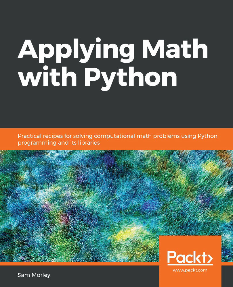
You're reading from   Applying Math with Python Practical recipes for solving computational math problems using Python programming and its libraries

Arrow left icon
Product type Paperback
Published in Jul 2020
Publisher Packt
ISBN-13 9781838989750
Length 358 pages
Edition 1st Edition
Languages
Arrow right icon
Authors (2):
Arrow left icon
Sam Morley Sam Morley
Author Profile Icon Sam Morley
Sam Morley
Sam Morley Sam Morley
Author Profile Icon Sam Morley
Sam Morley
Arrow right icon
View More author details
Toc

Table of Contents (12) Chapters Close

Preface 1. Basic Packages, Functions, and Concepts 2. Mathematical Plotting with Matplotlib FREE CHAPTER 3. Calculus and Differential Equations 4. Working with Randomness and Probability 5. Working with Trees and Networks 6. Working with Data and Statistics 7. Regression and Forecasting 8. Geometric Problems 9. Finding Optimal Solutions 10. Miscellaneous Topics 11. Other Books You May Enjoy

Solving partial differential equations numerically

Partial differential equations are differential equations that involve partial derivatives of functions in two or more variables, as opposed to ordinary derivatives in only a single variable. Partial differential equations is a vast topic, and could easily fill a series of books. A typical example of a partial differential equation is the (one-dimensional) heat equation

where α is a positive constant and f(t, x) is a function. The solution to this partial differential equation is a function u(t, x), which represents the temperature of a rod, occupying the x range 0 ≤ x ≤ L, at a given time t > 0. To keep things simple, we will take f(t, x) = 0, which amounts to saying that no heating/cooling is applied to the system, α = 1, and L = 2. In practice, we can rescale the problem to fix the constant α, so this is not a restrictive problem. In this example, we will...

lock icon The rest of the chapter is locked
Register for a free Packt account to unlock a world of extra content!
A free Packt account unlocks extra newsletters, articles, discounted offers, and much more. Start advancing your knowledge today.
Unlock this book and the full library FREE for 7 days
Get unlimited access to 7000+ expert-authored eBooks and videos courses covering every tech area you can think of
Renews at $19.99/month. Cancel anytime
Banner background image