Search icon CANCEL
Arrow left icon
Explore Products
Best Sellers
New Releases
Books
Videos
Audiobooks
Learning Hub
Conferences
Free Learning
Arrow right icon
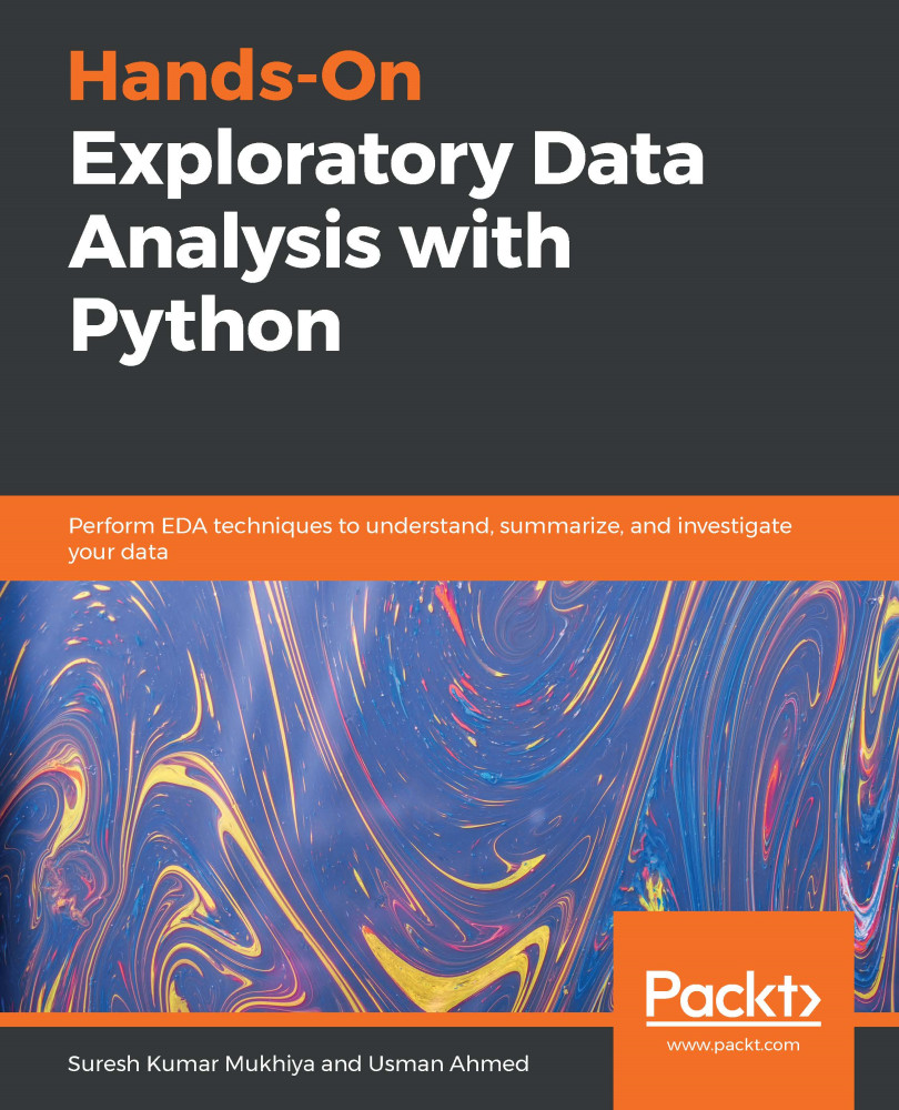
Hands-On Exploratory Data Analysis with Python

Hands-On Exploratory Data Analysis with Python: Perform EDA techniques to understand, summarize, and investigate your data

eBook
$63.99
Paperback
$79.99
Subscription
Free Trial
Renews at $19.99p/m

What do you get with eBook?

Product feature icon Instant access to your Digital eBook purchase
Product feature icon Download this book in EPUB and PDF formats
Product feature icon Access this title in our online reader with advanced features
Product feature icon DRM FREE - Read whenever, wherever and however you want
Product feature icon AI Assistant (beta) to help accelerate your learning
Table of content icon View table of contents Preview book icon Preview Book

Hands-On Exploratory Data Analysis with Python

Exploratory Data Analysis Fundamentals

The main objective of this introductory chapter is to revise the fundamentals of Exploratory Data Analysis (EDA), what it is, the key concepts of profiling and quality assessment, the main dimensions of EDA, and the main challenges and opportunities in EDA.

Data encompasses a collection of discrete objects, numbers, words, events, facts, measurements, observations, or even descriptions of things. Such data is collected and stored by every event or process occurring in several disciplines, including biology, economics, engineering, marketing, and others. Processing such data elicits useful information and processing such information generates useful knowledge. But an important question is: how can we generate meaningful and useful information from such data? An answer to this question is EDA. EDA is a process of examining the available dataset to discover patterns, spot anomalies, test hypotheses, and check assumptions using statistical measures. In this chapter, we are going to discuss the steps involved in performing top-notch exploratory data analysis and get our hands dirty using some open source databases.

As mentioned here and in several studies, the primary aim of EDA is to examine what data can tell us before actually going through formal modeling or hypothesis formulation. John Tuckey promoted EDA to statisticians to examine and discover the data and create newer hypotheses that could be used for the development of a newer approach in data collection and experimentations.

In this chapter, we are going to learn and revise the following topics:

  • Understanding data science
  • The significance of EDA
  • Making sense of data
  • Comparing EDA with classical and Bayesian analysis
  • Software tools available for EDA
  • Getting started with EDA

Understanding data science

Let's get this out of the way by pointing out that, if you have not heard about data science, then you should not be reading this book. Everyone right now is talking about data science in one way or another. Data science is at the peak of its hype and the skills for data scientists are changing. Now, data scientists are not only required to build a performant model, but it is essential for them to explain the results obtained and use the result for business intelligence. During my talks, seminars, and presentations, I find several people trying to ask me: what type of skillset do I need to learn in order to become a top-notch data scientist? Do I need to get a Ph.D. in data science? Well, one thing I could tell you straight away is you do not need a Ph.D. to be an expert in data science. But one thing that people generally agree on is that data science involves cross-disciplinary knowledge from computer science, data, statistics, and mathematics. There are several phases of data analysis, including data requirements, data collection, data processing, data cleaning, exploratory data analysis, modeling and algorithms, and data product and communication. These phases are similar to the CRoss-Industry Standard Process for data mining (CRISP) framework in data mining.

The main takeaway here is the stages of EDA, as it is an important aspect of data analysis and data mining. Let's understand in brief what these stages are:

  • Data requirements: There can be various sources of data for an organization. It is important to comprehend what type of data is required for the organization to be collected, curated, and stored. For example, an application tracking the sleeping pattern of patients suffering from dementia requires several types of sensors' data storage, such as sleep data, heart rate from the patient, electro-dermal activities, and user activities pattern. All of these data points are required to correctly diagnose the mental state of the person. Hence, these are mandatory requirements for the application. In addition to this, it is required to categorize the data, numerical or categorical, and the format of storage and dissemination.
  • Data collection: Data collected from several sources must be stored in the correct format and transferred to the right information technology personnel within a company. As mentioned previously, data can be collected from several objects on several events using different types of sensors and storage tools.
  • Data processing: Preprocessing involves the process of pre-curating the dataset before actual analysis. Common tasks involve correctly exporting the dataset, placing them under the right tables, structuring them, and exporting them in the correct format.
  • Data cleaning: Preprocessed data is still not ready for detailed analysis. It must be correctly transformed for an incompleteness check, duplicates check, error check, and missing value check. These tasks are performed in the data cleaning stage, which involves responsibilities such as matching the correct record, finding inaccuracies in the dataset, understanding the overall data quality, removing duplicate items, and filling in the missing values. However, how could we identify these anomalies on any dataset? Finding such data issues requires us to perform some analytical techniques. We will be learning several such analytical techniques in Chapter 4, Data Transformation. To understand briefly, data cleaning is dependent on the types of data under study. Hence, it is most essential for data scientists or EDA experts to comprehend different types of datasets. An example of data cleaning would be using outlier detection methods for quantitative data cleaning.
  • EDA: Exploratory data analysis, as mentioned before, is the stage where we actually start to understand the message contained in the data. It should be noted that several types of data transformation techniques might be required during the process of exploration. We will cover descriptive statistics in-depth in Section 2, Chapter 5, Descriptive Statistics, to understand the mathematical foundation behind descriptive statistics. This entire book is dedicated to tasks involved in exploratory data analysis.
  • Modeling and algorithm: From a data science perspective, generalized models or mathematical formulas can represent or exhibit relationships among different variables, such as correlation or causation. These models or equations involve one or more variables that depend on other variables to cause an event. For example, when buying, say, pens, the total price of pens(Total) = price for one pen(UnitPrice) * the number of pens bought (Quantity). Hence, our model would be Total = UnitPrice * Quantity. Here, the total price is dependent on the unit price. Hence, the total price is referred to as the dependent variable and the unit price is referred to as an independent variable. In general, a model always describes the relationship between independent and dependent variables. Inferential statistics deals with quantifying relationships between particular variables.
    The Judd model for describing the relationship between data, model, and error still holds true: Data = Model + Error. We will discuss in detail model development in Section 3, Chapter 10, Model Evaluation. An example of inferential statistics would be regression analysis. We will discuss regression analysis in Chapter 9, Regression.
  • Data Product: Any computer software that uses data as inputs, produces outputs, and provides feedback based on the output to control the environment is referred to as a data product. A data product is generally based on a model developed during data analysis, for example, a recommendation model that inputs user purchase history and recommends a related item that the user is highly likely to buy.
  • Communication: This stage deals with disseminating the results to end stakeholders to use the result for business intelligence. One of the most notable steps in this stage is data visualization. Visualization deals with information relay techniques such as tables, charts, summary diagrams, and bar charts to show the analyzed result. We will outline several visualization techniques in Chapter 2, Visual Aids for EDA, with different types of data.

The significance of EDA

Different fields of science, economics, engineering, and marketing accumulate and store data primarily in electronic databases. Appropriate and well-established decisions should be made using the data collected. It is practically impossible to make sense of datasets containing more than a handful of data points without the help of computer programs. To be certain of the insights that the collected data provides and to make further decisions, data mining is performed where we go through distinctive analysis processes. Exploratory data analysis is key, and usually the first exercise in data mining. It allows us to visualize data to understand it as well as to create hypotheses for further analysis. The exploratory analysis centers around creating a synopsis of data or insights for the next steps in a data mining project.

EDA actually reveals ground truth about the content without making any underlying assumptions. This is the fact that data scientists use this process to actually understand what type of modeling and hypotheses can be created. Key components of exploratory data analysis include summarizing data, statistical analysis, and visualization of data. Python provides expert tools for exploratory analysis, with pandas for summarizing; scipy, along with others, for statistical analysis; and matplotlib and plotly for visualizations.

That makes sense, right? Of course it does. That is one of the reasons why you are going through this book. After understanding the significance of EDA, let's discover what are the most generic steps involved in EDA in the next section.

Steps in EDA

Having understood what EDA is, and its significance, let's understand the various steps involved in data analysis. Basically, it involves four different steps. Let's go through each of them to get a brief understanding of each step:

  • Problem definition: Before trying to extract useful insight from the data, it is essential to define the business problem to be solved. The problem definition works as the driving force for a data analysis plan execution. The main tasks involved in problem definition are defining the main objective of the analysis, defining the main deliverables, outlining the main roles and responsibilities, obtaining the current status of the data, defining the timetable, and performing cost/benefit analysis. Based on such a problem definition, an execution plan can be created.
  • Data preparation: This step involves methods for preparing the dataset before actual analysis. In this step, we define the sources of data, define data schemas and tables, understand the main characteristics of the data, clean the dataset, delete non-relevant datasets, transform the data, and divide the data into required chunks for analysis.
  • Data analysis: This is one of the most crucial steps that deals with descriptive statistics and analysis of the data. The main tasks involve summarizing the data, finding the hidden correlation and relationships among the data, developing predictive models, evaluating the models, and calculating the accuracies. Some of the techniques used for data summarization are summary tables, graphs, descriptive statistics, inferential statistics, correlation statistics, searching, grouping, and mathematical models.
  • Development and representation of the results: This step involves presenting the dataset to the target audience in the form of graphs, summary tables, maps, and diagrams. This is also an essential step as the result analyzed from the dataset should be interpretable by the business stakeholders, which is one of the major goals of EDA. Most of the graphical analysis techniques include scattering plots, character plots, histograms, box plots, residual plots, mean plots, and others. We will explore several types of graphical representation in Chapter 2, Visual Aids for EDA.

Making sense of data

It is crucial to identify the type of data under analysis. In this section, we are going to learn about different types of data that you can encounter during analysis. Different disciplines store different kinds of data for different purposes. For example, medical researchers store patients' data, universities store students' and teachers' data, and real estate industries storehouse and building datasets. A dataset contains many observations about a particular object. For instance, a dataset about patients in a hospital can contain many observations. A patient can be described by a patient identifier (ID), name, address, weight, date of birth, address, email, and gender. Each of these features that describes a patient is a variable. Each observation can have a specific value for each of these variables. For example, a patient can have the following:

PATIENT_ID = 1001
Name = Yoshmi Mukhiya
Address = Mannsverk 61, 5094, Bergen, Norway
Date of birth = 10th July 2018
Email = yoshmimukhiya@gmail.com
Weight = 10
Gender = Female

These datasets are stored in hospitals and are presented for analysis. Most of this data is stored in some sort of database management system in tables/schema. An example of a table for storing patient information is shown here:

PATIENT_ID

NAME

ADDRESS

DOB

EMAIL

Gender

WEIGHT

001

Suresh Kumar Mukhiya

Mannsverk, 61

30.12.1989

skmu@hvl.no

Male

68

002

Yoshmi Mukhiya

Mannsverk 61, 5094, Bergen

10.07.2018

yoshmimukhiya@gmail.com

Female

1

003

Anju Mukhiya

Mannsverk 61, 5094, Bergen

10.12.1997

anjumukhiya@gmail.com

Female

24

004

Asha Gaire

Butwal, Nepal

30.11.1990

aasha.gaire@gmail.com

Female

23

005

Ola Nordmann

Danmark, Sweden

12.12.1789

ola@gmail.com

Male

75

To summarize the preceding table, there are four observations (001, 002, 003, 004, 005). Each observation describes variables (PatientID, name, address, dob, email, gender, and weight). Most of the dataset broadly falls into two groups—numerical data and categorical data.

Numerical data

This data has a sense of measurement involved in it; for example, a person's age, height, weight, blood pressure, heart rate, temperature, number of teeth, number of bones, and the number of family members. This data is often referred to as quantitative data in statistics. The numerical dataset can be either discrete or continuous types.

Discrete data

This is data that is countable and its values can be listed out. For example, if we flip a coin, the number of heads in 200 coin flips can take values from 0 to 200 (finite) cases. A variable that represents a discrete dataset is referred to as a discrete variable. The discrete variable takes a fixed number of distinct values. For example, the Country variable can have values such as Nepal, India, Norway, and Japan. It is fixed. The Rank variable of a student in a classroom can take values from 1, 2, 3, 4, 5, and so on.

Continuous data

A variable that can have an infinite number of numerical values within a specific range is classified as continuous data. A variable describing continuous data is a continuous variable. For example, what is the temperature of your city today? Can we be finite? Similarly, the weight variable in the previous section is a continuous variable. We are going to use a car dataset in Chapter 5, Descriptive Statistics, to perform EDA.

A section of the table is shown in the following table:

Check the preceding table and determine which of the variables are discrete and which of the variables are continuous. Can you justify your claim? Continuous data can follow an interval measure of scale or ratio measure of scale. We will go into more detail in the Measurement scales section in this chapter.

Categorical data

This type of data represents the characteristics of an object; for example, gender, marital status, type of address, or categories of the movies. This data is often referred to as qualitative datasets in statistics. To understand clearly, here are some of the most common types of categorical data you can find in data:

  • Gender (Male, Female, Other, or Unknown)
  • Marital Status (Annulled, Divorced, Interlocutory, Legally Separated, Married, Polygamous, Never Married, Domestic Partner, Unmarried, Widowed, or Unknown)
  • Movie genres (Action, Adventure, Comedy, Crime, Drama, Fantasy, Historical, Horror, Mystery, Philosophical, Political, Romance, Saga, Satire, Science Fiction, Social, Thriller, Urban, or Western)
  • Blood type (A, B, AB, or O)
  • Types of drugs (Stimulants, Depressants, Hallucinogens, Dissociatives, Opioids, Inhalants, or Cannabis)

A variable describing categorical data is referred to as a categorical variable. These types of variables can have one of a limited number of values. It is easier for computer science students to understand categorical values as enumerated types or enumerations of variables. There are different types of categorical variables:

  • A binary categorical variable can take exactly two values and is also referred to as a dichotomous variable. For example, when you create an experiment, the result is either success or failure. Hence, results can be understood as a binary categorical variable.
  • Polytomous variables are categorical variables that can take more than two possible values. For example, marital status can have several values, such as annulled, divorced, interlocutory, legally separated, married, polygamous, never married, domestic partners, unmarried, widowed, domestic partner, and unknown. Since marital status can take more than two possible values, it is a polytomous variable.

Most of the categorical dataset follows either nominal or ordinal measurement scales. Let's understand what is a nominal or ordinal scale in the next section.

Measurement scales

There are four different types of measurement scales described in statistics: nominal, ordinal, interval, and ratio. These scales are used more in academic industries. Let's understand each of them with some examples.

Nominal

These are practiced for labeling variables without any quantitative value. The scales are generally referred to as labels. And these scales are mutually exclusive and do not carry any numerical importance. Let's see some examples:

  • What is your gender?
  • Male
  • Female
  • Third gender/Non-binary
  • I prefer not to answer
  • Other
  • Other examples include the following:
  • The languages that are spoken in a particular country
  • Biological species
  • Parts of speech in grammar (noun, pronoun, adjective, and so on)
  • Taxonomic ranks in biology (Archea, Bacteria, and Eukarya)

Nominal scales are considered qualitative scales and the measurements that are taken using qualitative scales are considered qualitative data. However, the advancement in qualitative research has created confusion to be definitely considered as qualitative. If, for example, someone uses numbers as labels in the nominal measurement sense, they have no concrete numerical value or meaning. No form of arithmetic calculation can be made on nominal measures.

You might be thinking why should you care about whether data is nominal or ordinal? Should we not just start loading the data and begin our analysis? Well, we could. But think about this: you have a dataset, and you want to analyze it. How will you decide whether you can make a pie chart, bar chart, or histogram? Are you getting my point?

Well, for example, in the case of a nominal dataset, you can certainly know the following:

  • Frequency is the rate at which a label occurs over a period of time within the dataset.
  • Proportion can be calculated by dividing the frequency by the total number of events.
  • Then, you could compute the percentage of each proportion.
  • And to visualize the nominal dataset, you can use either a pie chart or a bar chart.

If you know your data follows nominal scales, you can use a pie chart or bar chart. That's one less thing to worry about, right? My point is, understanding the type of data is relevant in understanding what type of computation you can perform, what type of model you should fit on the dataset, and what type of visualization you can generate.

Ordinal

The main difference in the ordinal and nominal scale is the order. In ordinal scales, the order of the values is a significant factor. An easy tip to remember the ordinal scale is that it sounds like an order. Have you heard about the Likert scale, which uses a variation of an ordinal scale? Let's check an example of ordinal scale using the Likert scale: WordPress is making content managers' lives easier. How do you feel about this statement? The following diagram shows the Likert scale:

As depicted in the preceding diagram, the answer to the question of WordPress is making content managers' lives easier is scaled down to five different ordinal values, Strongly Agree, Agree, Neutral, Disagree, and Strongly Disagree. Scales like these are referred to as the Likert scale. Similarly, the following diagram shows more examples of the Likert scale:

To make it easier, consider ordinal scales as an order of ranking (1st, 2nd, 3rd, 4th, and so on). The median item is allowed as the measure of central tendency; however, the average is not permitted.

Interval

In interval scales, both the order and exact differences between the values are significant. Interval scales are widely used in statistics, for example, in the measure of central tendencies—mean, median, mode, and standard deviations. Examples include location in Cartesian coordinates and direction measured in degrees from magnetic north. The mean, median, and mode are allowed on interval data.

Ratio

Ratio scales contain order, exact values, and absolute zero, which makes it possible to be used in descriptive and inferential statistics. These scales provide numerous possibilities for statistical analysis. Mathematical operations, the measure of central tendencies, and the measure of dispersion and coefficient of variation can also be computed from such scales.

Examples include a measure of energy, mass, length, duration, electrical energy, plan angle, and volume. The following table gives a summary of the data types and scale measures:

In the next section, we will compare EDA with classical and Bayesian analysis.

Comparing EDA with classical and Bayesian analysis

There are several approaches to data analysis. The most popular ones that are relevant to this book are the following:

  • Classical data analysis: For the classical data analysis approach, the problem definition and data collection step are followed by model development, which is followed by analysis and result communication.
  • Exploratory data analysis approach: For the EDA approach, it follows the same approach as classical data analysis except the model imposition and the data analysis steps are swapped. The main focus is on the data, its structure, outliers, models, and visualizations. Generally, in EDA, we do not impose any deterministic or probabilistic models on the data.
  • Bayesian data analysis approach: The Bayesian approach incorporates prior probability distribution knowledge into the analysis steps as shown in the following diagram. Well, simply put, prior probability distribution of any quantity expresses the belief about that particular quantity before considering some evidence. Are you still lost with the term prior probability distribution? Andrew Gelman has a very descriptive paper about prior probability distribution. The following diagram shows three different approaches for data analysis illustrating the difference in their execution steps:

Data analysts and data scientists freely mix steps mentioned in the preceding approaches to get meaningful insights from the data. In addition to that, it is essentially difficult to judge or estimate which model is best for data analysis. All of them have their paradigms and are suitable for different types of data analysis.

Software tools available for EDA

There are several software tools that are available to facilitate EDA. Here, we are going to outline some of the open source tools:

  • Python: This is an open source programming language widely used in data analysis, data mining, and data science (https://www.python.org/). For this book, we will be using Python.
  • R programming language: R is an open source programming language that is widely utilized in statistical computation and graphical data analysis (https://www.r-project.org).
  • Weka: This is an open source data mining package that involves several EDA tools and algorithms (https://www.cs.waikato.ac.nz/ml/weka/).
  • KNIME: This is an open source tool for data analysis and is based on Eclipse (https://www.knime.com/).

Getting started with EDA

As mentioned earlier, we are going to use Python as the main tool for data analysis. Yay! Well, if you ask me why, Python has been consistently ranked among the top 10 programming languages and is widely adopted for data analysis and data mining by data science experts. In this book, we assume you have a working knowledge of Python. If you are not familiar with Python, it's probably too early to get started with data analysis. I assume you are familiar with the following Python tools and packages:

Python programming

Fundamental concepts of variables, string, and data types

Conditionals and functions

Sequences, collections, and iterations

Working with files

Object-oriented programming

NumPy

Create arrays with NumPy, copy arrays, and divide arrays

Perform different operations on NumPy arrays

Understand array selections, advanced indexing, and expanding

Working with multi-dimensional arrays

Linear algebraic functions and built-in NumPy functions

pandas

Understand and create DataFrame objects

Subsetting data and indexing data

Arithmetic functions, and mapping with pandas

Managing index

Building style for visual analysis

Matplotlib

Loading linear datasets

Adjusting axes, grids, labels, titles, and legends

Saving plots

SciPy

Importing the package

Using statistical packages from SciPy

Performing descriptive statistics

Inference and data analysis

Before diving into details about analysis, we need to make sure we are on the same page. Let's go through the checklist and verify that you meet all of the prerequisites to get the best out of this book:

Setting up a virtual environment

> pip install virtualenv
> virtualenv Local_Version_Directory -p Python_System_Directory

Reading/writing to files

filename = "datamining.txt" 
file = open(filename, mode="r", encoding='utf-8')
for line in file:
lines = file.readlines()
print(lines)
file.close()

Error handling

try:
Value = int(input("Type a number between 47 and 100:"))
except ValueError:
print("You must type a number between 47 and 100!")
else:
if (Value > 47) and (Value <= 100):
print("You typed: ", Value)
else:
print("The value you typed is incorrect!")

Object-oriented concept

class Disease:
def __init__(self, disease = 'Depression'):
self.type = disease

def getName(self):
print("Mental Health Diseases: {0}".format(self.type))

d1 = Disease('Social Anxiety Disorder')
d1.getName()

Next, let's look at the basic operations of EDA using the NumPy library.

NumPy

In this section, we are going to revise the basic operations of EDA using the NumPy library. If you are familiar with these operations, feel free to jump to the next section. It might feel obvious when going through the code, but it is essential to make sure you understand these concepts before digging into EDA operations. When I started learning data science approaches, I followed a lot of blogs where they just reshaped an array or matrix. When I ran their code, it worked fine, but I never understood how I was able to add two matrices of different dimensions. In this section, I have tried to explicitly point out some of the basic numpy operations:

  • For importing numpy, we will use the following code:
import numpy as np
  • For creating different types of numpy arrays, we will use the following code:
# importing numpy
import numpy as np

# Defining 1D array
my1DArray = np.array([1, 8, 27, 64])
print(my1DArray)

# Defining and printing 2D array
my2DArray = np.array([[1, 2, 3, 4], [2, 4, 9, 16], [4, 8, 18, 32]])
print(my2DArray)

#Defining and printing 3D array
my3Darray = np.array([[[ 1, 2 , 3 , 4],[ 5 , 6 , 7 ,8]], [[ 1, 2, 3, 4],[ 9, 10, 11, 12]]])
print(my3Darray)
  • For displaying basic information, such as the data type, shape, size, and strides of a NumPy array, we will use the following code:
# Print out memory address
print(my2DArray.data)

# Print the shape of array
print(my2DArray.shape)

# Print out the data type of the array
print(my2DArray.dtype)

# Print the stride of the array.
print(my2DArray.strides)
  • For creating an array using built-in NumPy functions, we will use the following code:
# Array of ones
ones = np.ones((3,4))
print(ones)

# Array of zeros
zeros = np.zeros((2,3,4),dtype=np.int16)
print(zeros)

# Array with random values
np.random.random((2,2))

# Empty array
emptyArray = np.empty((3,2))
print(emptyArray)

# Full array
fullArray = np.full((2,2),7)
print(fullArray)

# Array of evenly-spaced values
evenSpacedArray = np.arange(10,25,5)
print(evenSpacedArray)

# Array of evenly-spaced values
evenSpacedArray2 = np.linspace(0,2,9)
print(evenSpacedArray2)
  • For NumPy arrays and file operations, we will use the following code:
# Save a numpy array into file
x = np.arange(0.0,50.0,1.0)
np.savetxt('data.out', x, delimiter=',')

# Loading numpy array from text
z = np.loadtxt('data.out', unpack=True)
print(z)

# Loading numpy array using genfromtxt method
my_array2 = np.genfromtxt('data.out',
skip_header=1,
filling_values=-999)
print(my_array2)
  • For inspecting NumPy arrays, we will use the following code:
# Print the number of `my2DArray`'s dimensions
print(my2DArray.ndim)

# Print the number of `my2DArray`'s elements
print(my2DArray.size)

# Print information about `my2DArray`'s memory layout
print(my2DArray.flags)

# Print the length of one array element in bytes
print(my2DArray.itemsize)

# Print the total consumed bytes by `my2DArray`'s elements
print(my2DArray.nbytes)
  • Broadcasting is a mechanism that permits NumPy to operate with arrays of different shapes when performing arithmetic operations:
# Rule 1: Two dimensions are operatable if they are equal
# Create an array of two dimension
A =np.ones((6, 8))

# Shape of A
print(A.shape)

# Create another array
B = np.random.random((6,8))

# Shape of B
print(B.shape)

# Sum of A and B, here the shape of both the matrix is same.
print(A + B)

Secondly, two dimensions are also compatible when one of the dimensions of the array is 1. Check the example given here:

# Rule 2: Two dimensions are also compatible when one of them is 1
# Initialize `x`
x = np.ones((3,4))
print(x)

# Check shape of `x`
print(x.shape)

# Initialize `y`
y = np.arange(4)
print(y)

# Check shape of `y`
print(y.shape)

# Subtract `x` and `y`
print(x - y)

Lastly, there is a third rule that says two arrays can be broadcast together if they are compatible in all of the dimensions. Check the example given here:

# Rule 3: Arrays can be broadcast together if they are compatible in all dimensions
x = np.ones((6,8))
y = np.random.random((10, 1, 8))
print(x + y)

The dimensions of x(6,8) and y(10,1,8) are different. However, it is possible to add them. Why is that? Also, change y(10,2,8) or y(10,1,4) and it will give ValueError. Can you find out why? (Hint: check rule 1).

  • For seeing NumPy mathematics at work, we will use the following example:
# Basic operations (+, -, *, /, %)
x = np.array([[1, 2, 3], [2, 3, 4]])
y = np.array([[1, 4, 9], [2, 3, -2]])

# Add two array
add = np.add(x, y)
print(add)

# Subtract two array
sub = np.subtract(x, y)
print(sub)

# Multiply two array
mul = np.multiply(x, y)
print(mul)

# Divide x, y
div = np.divide(x,y)
print(div)

# Calculated the remainder of x and y
rem = np.remainder(x, y)
print(rem)
  • Let's now see how we can create a subset and slice an array using an index:
x = np.array([10, 20, 30, 40, 50])

# Select items at index 0 and 1
print(x[0:2])

# Select item at row 0 and 1 and column 1 from 2D array
y = np.array([[ 1, 2, 3, 4], [ 9, 10, 11 ,12]])
print(y[0:2, 1])

# Specifying conditions
biggerThan2 = (y >= 2)
print(y[biggerThan2])

Next, we will use the pandas library to gain insights from data.

Pandas

Wes McKinney open sourced the pandas library (https://github.com/wesm) that has been widely used in data science. We will be utilizing this library to get meaningful insight from the data. Before delving in detail into this section, we are going to revisit some of the most fundamental techniques in pandas that you should be familiar with so as to be able to follow upcoming chapters. If these things are new to you, feel free to check one of the further reading sections for additional resources. Perform the following steps:

  1. Use the following to set default parameters:
import numpy as np
import pandas as pd
print("Pandas Version:", pd.__version__)

pd.set_option('display.max_columns', 500)
pd.set_option('display.max_rows', 500)
  1. In pandas, we can create data structures in two ways: series and dataframes. Check the following snippet to understand how we can create a dataframe from series, dictionary, and n-dimensional arrays.

The following code snippet shows how we can create a dataframe from a series:

series = pd.Series([2, 3, 7, 11, 13, 17, 19, 23])
print(series)

# Creating dataframe from Series
series_df = pd.DataFrame({
'A': range(1, 5),
'B': pd.Timestamp('20190526'),
'C': pd.Series(5, index=list(range(4)), dtype='float64'),
'D': np.array([3] * 4, dtype='int64'),
'E': pd.Categorical(["Depression", "Social Anxiety", "Bipolar Disorder", "Eating Disorder"]),
'F': 'Mental health',
'G': 'is challenging'
})
print(series_df)

The following code snippet shows how to create a dataframe for a dictionary:

# Creating dataframe from Dictionary
dict_df = [{'A': 'Apple', 'B': 'Ball'},{'A': 'Aeroplane', 'B': 'Bat', 'C': 'Cat'}]
dict_df = pd.DataFrame(dict_df)
print(dict_df)

The following code snippet shows how to create a dataframe from n-dimensional arrays:

# Creating a dataframe from ndarrays
sdf = {
'County':['Østfold', 'Hordaland', 'Oslo', 'Hedmark', 'Oppland', 'Buskerud'],
'ISO-Code':[1,2,3,4,5,6],
'Area': [4180.69, 4917.94, 454.07, 27397.76, 25192.10, 14910.94],
'Administrative centre': ["Sarpsborg", "Oslo", "City of Oslo", "Hamar", "Lillehammer", "Drammen"]
}
sdf = pd.DataFrame(sdf)
print(sdf)
  1. Now, let's load a dataset from an external source into a pandas DataFrame. After that, let's see the first 10 entries:

columns = ['age', 'workclass', 'fnlwgt', 'education', 'education_num',
'marital_status', 'occupation', 'relationship', 'ethnicity', 'gender','capital_gain','capital_loss','hours_per_week','country_of_origin','income']
df = pd.read_csv('http://archive.ics.uci.edu/ml/machine-learning-databases/adult/adult.data',names=columns)
df.head(10)

If you run the preceding cell, you should get an output similar to the following screenshot:

  1. The following code displays the rows, columns, data types, and memory used by the dataframe:
df.info()

The output of the preceding code snippet should be similar to the following:

# Output:
<class 'pandas.core.frame.DataFrame'>
RangeIndex: 32561 entries, 0 to 32560
Data columns (total 15 columns):
age 32561 non-null int64
workclass 32561 non-null object
fnlwgt 32561 non-null int64
education 32561 non-null object
education_num 32561 non-null int64
marital_status 32561 non-null object
occupation 32561 non-null object
relationship 32561 non-null object
ethnicity 32561 non-null object
gender 32561 non-null object
capital_gain 32561 non-null int64
capital_loss 32561 non-null int64
hours_per_week 32561 non-null int64
country_of_origin 32561 non-null object
income 32561 non-null object
dtypes: int64(6), object(9)
memory usage: 3.7+ MB
  1. Let's now see how we can select rows and columns in any dataframe:
# Selects a row
df.iloc[10]

# Selects 10 rows
df.iloc[0:10]

# Selects a range of rows
df.iloc[10:15]

# Selects the last 2 rows
df.iloc[-2:]

# Selects every other row in columns 3-5
df.iloc[::2, 3:5].head()
  1. Let's combine NumPy and pandas to create a dataframe as follows:
import pandas as pd
import numpy as np

np.random.seed(24)
dFrame = pd.DataFrame({'F': np.linspace(1, 10, 10)})
dFrame = pd.concat([df, pd.DataFrame(np.random.randn(10, 5), columns=list('EDCBA'))],
axis=1)
dFrame.iloc[0, 2] = np.nan
dFrame

It should produce a dataframe table similar to the following screenshot:

  1. Let's style this table using a custom rule. If the values are greater than zero, we change the color to black (the default color); if the value is less than zero, we change the color to red; and finally, everything else would be colored green. Let's define a Python function to accomplish that:
# Define a function that should color the values that are less than 0 
def colorNegativeValueToRed(value):
if value < 0:
color = 'red'
elif value > 0:
color = 'black'
else:
color = 'green'

return 'color: %s' % color
  1. Now, let's pass this function to the dataframe. We can do this by using the style method provided by pandas inside the dataframe:
s = df.style.applymap(colorNegativeValueToRed, subset=['A','B','C','D','E'])
s

It should display a colored dataframe as shown in the following screenshot:

It should be noted that the applymap and apply methods are computationally expensive as they apply to each value inside the dataframe. Hence, it will take some time to execute. Have patience and await execution.

  1. Now, let's go one step deeper. We want to scan each column and highlight the maximum value and the minimum value in that column:
def highlightMax(s):
isMax = s == s.max()
return ['background-color: orange' if v else '' for v in isMax]

def highlightMin(s):
isMin = s == s.min()
return ['background-color: green' if v else '' for v in isMin]

We apply these two functions to the dataframe as follows:

df.style.apply(highlightMax).apply(highlightMin).highlight_null(null_color='red')

The output should be similar to the following screenshot:

  1. Are you still not happy with your visualization? Let's try to use another Python library called seaborn and provide a gradient to the table:
import seaborn as sns

colorMap = sns.light_palette("pink", as_cmap=True)

styled = df.style.background_gradient(cmap=colorMap)
styled

The dataframe should have an orange gradient applied to it:

There are endless possibilities. How you present your result depends on you. Keep in mind that when you present your results to end stakeholders (your managers, boss, or non-technical persons), no matter how intelligently written your code is, it is worthless to them if they cannot make sense of your program. It is widely accepted that better-visualized results are easy to market.

SciPy

SciPy is a scientific library for Python and is open source. We are going to use this library in the upcoming chapters. This library depends on the NumPy library, which provides an efficient n-dimensional array manipulation function. We are going to learn more about these libraries in the upcoming chapters. My intention here is just to inform you to get prepared to face other libraries apart from NumPy and pandas. If you want to get started early, check for scipy.stats from the SciPy library.

Matplotlib

Matplotlib provides a huge library of customizable plots, along with a comprehensive set of backends. It can be utilized to create professional reporting applications, interactive analytical applications, complex dashboard applications, web/GUI applications, embedded views, and many more. We are going to explore Matplotlib in detail in Chapter 2, Visual Aids for EDA.

Summary

In this chapter, we revisited the most fundamental theory behind data analysis and exploratory data analysis. EDA is one of the most prominent steps in data analysis and involves steps such as data requirements, data collection, data processing, data cleaning, exploratory data analysis, modeling and algorithms, data production, and communication. It is crucial to identify the type of data under analysis. Different disciplines store different kinds of data for different purposes. For example, medical researchers store patients' data, universities store students' and teachers' data, real estate industries store house and building datasets, and many more. A dataset contains many observations about a particular object. Most of the datasets can be divided into numerical data and categorical datasets. There are four types of data measurement scales: nominal, ordinal, interval, and ratio.

We are going to use several Python libraries, including NumPy, pandas, SciPy, and Matplotlib, in this book for performing simple to complex exploratory data analysis. In the next chapter, we are going to learn about various types of visualization aids for exploratory data analysis.

Further reading

  • Myatt, Glenn J. (2006). Making Sense of Data: A Practical Guide to Exploratory Data Analysis and Data Mining. Print ISBN:9780470074718 |Online ISBN:9780470101025 |DOI:10.1002/0470101024
  • Chatfield, C. (1995). Problem Solving: A Statistician's Guide (2nd ed.). Chapman and Hall. ISBN 978-0412606304.
  • Prior distribution, Andrew Gelman Volume 3, pp 1634–1637, http://www.stat.columbia.edu/~gelman/research/published/p039-_o.pdf
  • Shearer, C. (2000). The CRISP-DM model: the new blueprint for data mining. J Data Warehousing; 5:13—22.
  • Judd, Charles and McCleland, Gary (1989). Data Analysis. Harcourt Brace Jovanovich. ISBN 0-15-516765-0.
  • Carifio, James and Perla, Rocco J. (2007). Ten Common Misunderstandings, Misconceptions, Persistent Myths, and Urban Legends about Likert Scales and Likert Response Formats and Their Antidotes. Journal of Social Sciences. 3 (3): 106–116. DOI:10.3844/jssp.2007.106.116
Left arrow icon Right arrow icon
Download code icon Download Code

Key benefits

  • Understand the fundamental concepts of exploratory data analysis using Python
  • Find missing values in your data and identify the correlation between different variables
  • Practice graphical exploratory analysis techniques using Matplotlib and the Seaborn Python package

Description

Exploratory Data Analysis (EDA) is an approach to data analysis that involves the application of diverse techniques to gain insights into a dataset. This book will help you gain practical knowledge of the main pillars of EDA - data cleaning, data preparation, data exploration, and data visualization. You’ll start by performing EDA using open source datasets and perform simple to advanced analyses to turn data into meaningful insights. You’ll then learn various descriptive statistical techniques to describe the basic characteristics of data and progress to performing EDA on time-series data. As you advance, you’ll learn how to implement EDA techniques for model development and evaluation and build predictive models to visualize results. Using Python for data analysis, you’ll work with real-world datasets, understand data, summarize its characteristics, and visualize it for business intelligence. By the end of this EDA book, you’ll have developed the skills required to carry out a preliminary investigation on any dataset, yield insights into data, present your results with visual aids, and build a model that correctly predicts future outcomes.

Who is this book for?

This EDA book is for anyone interested in data analysis, especially students, statisticians, data analysts, and data scientists. The practical concepts presented in this book can be applied in various disciplines to enhance decision-making processes with data analysis and synthesis. Fundamental knowledge of Python programming and statistical concepts is all you need to get started with this book.

What you will learn

  • Import, clean, and explore data to perform preliminary analysis using powerful Python packages
  • Identify and transform erroneous data using different data wrangling techniques
  • Explore the use of multiple regression to describe non-linear relationships
  • Discover hypothesis testing and explore techniques of time-series analysis
  • Understand and interpret results obtained from graphical analysis
  • Build, train, and optimize predictive models to estimate results
  • Perform complex EDA techniques on open source datasets

Product Details

Country selected
Publication date, Length, Edition, Language, ISBN-13
Publication date : Mar 27, 2020
Length: 352 pages
Edition : 1st
Language : English
ISBN-13 : 9781789535624
Category :
Languages :
Concepts :
Tools :

What do you get with eBook?

Product feature icon Instant access to your Digital eBook purchase
Product feature icon Download this book in EPUB and PDF formats
Product feature icon Access this title in our online reader with advanced features
Product feature icon DRM FREE - Read whenever, wherever and however you want
Product feature icon AI Assistant (beta) to help accelerate your learning

Product Details

Publication date : Mar 27, 2020
Length: 352 pages
Edition : 1st
Language : English
ISBN-13 : 9781789535624
Category :
Languages :
Concepts :
Tools :

Packt Subscriptions

See our plans and pricing
Modal Close icon
$19.99 billed monthly
Feature tick icon Unlimited access to Packt's library of 7,000+ practical books and videos
Feature tick icon Constantly refreshed with 50+ new titles a month
Feature tick icon Exclusive Early access to books as they're written
Feature tick icon Solve problems while you work with advanced search and reference features
Feature tick icon Offline reading on the mobile app
Feature tick icon Simple pricing, no contract
$199.99 billed annually
Feature tick icon Unlimited access to Packt's library of 7,000+ practical books and videos
Feature tick icon Constantly refreshed with 50+ new titles a month
Feature tick icon Exclusive Early access to books as they're written
Feature tick icon Solve problems while you work with advanced search and reference features
Feature tick icon Offline reading on the mobile app
Feature tick icon Choose a DRM-free eBook or Video every month to keep
Feature tick icon PLUS own as many other DRM-free eBooks or Videos as you like for just $5 each
Feature tick icon Exclusive print discounts
$279.99 billed in 18 months
Feature tick icon Unlimited access to Packt's library of 7,000+ practical books and videos
Feature tick icon Constantly refreshed with 50+ new titles a month
Feature tick icon Exclusive Early access to books as they're written
Feature tick icon Solve problems while you work with advanced search and reference features
Feature tick icon Offline reading on the mobile app
Feature tick icon Choose a DRM-free eBook or Video every month to keep
Feature tick icon PLUS own as many other DRM-free eBooks or Videos as you like for just $5 each
Feature tick icon Exclusive print discounts

Frequently bought together


Stars icon
Total $ 167.97
Python Data Cleaning Cookbook
$48.99
Hands-On Exploratory Data Analysis with Python
$79.99
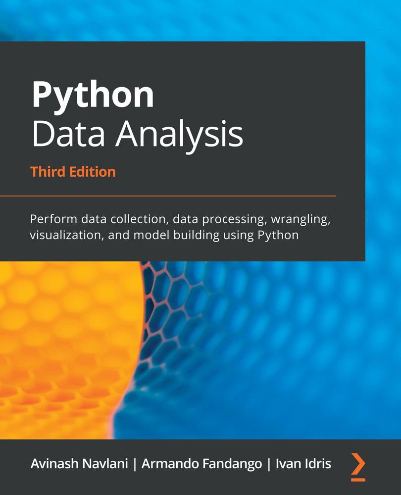
Python Data Analysis
$38.99
Total $ 167.97 Stars icon

Table of Contents

15 Chapters
Section 1: The Fundamentals of EDA Chevron down icon Chevron up icon
Exploratory Data Analysis Fundamentals Chevron down icon Chevron up icon
Visual Aids for EDA Chevron down icon Chevron up icon
EDA with Personal Email Chevron down icon Chevron up icon
Data Transformation Chevron down icon Chevron up icon
Section 2: Descriptive Statistics Chevron down icon Chevron up icon
Descriptive Statistics Chevron down icon Chevron up icon
Grouping Datasets Chevron down icon Chevron up icon
Correlation Chevron down icon Chevron up icon
Time Series Analysis Chevron down icon Chevron up icon
Section 3: Model Development and Evaluation Chevron down icon Chevron up icon
Hypothesis Testing and Regression Chevron down icon Chevron up icon
Model Development and Evaluation Chevron down icon Chevron up icon
EDA on Wine Quality Data Analysis Chevron down icon Chevron up icon
Other Books You May Enjoy Chevron down icon Chevron up icon

Customer reviews

Rating distribution
Full star icon Full star icon Half star icon Empty star icon Empty star icon 2.5
(2 Ratings)
5 star 0%
4 star 50%
3 star 0%
2 star 0%
1 star 50%
Denzel Ignatius Arulmani Selvam Oct 15, 2020
Full star icon Full star icon Full star icon Full star icon Empty star icon 4
Pros:1. Covers all the important concepts you need to know to get started with EDA.2. Lots of sample codes which the reader can use to get their hands dirty.3. Works excellently as a reference book to look up the basic concepts of EDA.Cons:This book only contains an brief overview of the concepts. So, if you want to get a very deep understanding of the subject matter, this is not the book for you.
Amazon Verified review Amazon
samarth saxena Aug 28, 2020
Full star icon Empty star icon Empty star icon Empty star icon Empty star icon 1
Worst print , black - white copy , no colour print as shown in Google book preview and not any special content
Amazon Verified review Amazon
Get free access to Packt library with over 7500+ books and video courses for 7 days!
Start Free Trial

FAQs

How do I buy and download an eBook? Chevron down icon Chevron up icon

Where there is an eBook version of a title available, you can buy it from the book details for that title. Add either the standalone eBook or the eBook and print book bundle to your shopping cart. Your eBook will show in your cart as a product on its own. After completing checkout and payment in the normal way, you will receive your receipt on the screen containing a link to a personalised PDF download file. This link will remain active for 30 days. You can download backup copies of the file by logging in to your account at any time.

If you already have Adobe reader installed, then clicking on the link will download and open the PDF file directly. If you don't, then save the PDF file on your machine and download the Reader to view it.

Please Note: Packt eBooks are non-returnable and non-refundable.

Packt eBook and Licensing When you buy an eBook from Packt Publishing, completing your purchase means you accept the terms of our licence agreement. Please read the full text of the agreement. In it we have tried to balance the need for the ebook to be usable for you the reader with our needs to protect the rights of us as Publishers and of our authors. In summary, the agreement says:

  • You may make copies of your eBook for your own use onto any machine
  • You may not pass copies of the eBook on to anyone else
How can I make a purchase on your website? Chevron down icon Chevron up icon

If you want to purchase a video course, eBook or Bundle (Print+eBook) please follow below steps:

  1. Register on our website using your email address and the password.
  2. Search for the title by name or ISBN using the search option.
  3. Select the title you want to purchase.
  4. Choose the format you wish to purchase the title in; if you order the Print Book, you get a free eBook copy of the same title. 
  5. Proceed with the checkout process (payment to be made using Credit Card, Debit Cart, or PayPal)
Where can I access support around an eBook? Chevron down icon Chevron up icon
  • If you experience a problem with using or installing Adobe Reader, the contact Adobe directly.
  • To view the errata for the book, see www.packtpub.com/support and view the pages for the title you have.
  • To view your account details or to download a new copy of the book go to www.packtpub.com/account
  • To contact us directly if a problem is not resolved, use www.packtpub.com/contact-us
What eBook formats do Packt support? Chevron down icon Chevron up icon

Our eBooks are currently available in a variety of formats such as PDF and ePubs. In the future, this may well change with trends and development in technology, but please note that our PDFs are not Adobe eBook Reader format, which has greater restrictions on security.

You will need to use Adobe Reader v9 or later in order to read Packt's PDF eBooks.

What are the benefits of eBooks? Chevron down icon Chevron up icon
  • You can get the information you need immediately
  • You can easily take them with you on a laptop
  • You can download them an unlimited number of times
  • You can print them out
  • They are copy-paste enabled
  • They are searchable
  • There is no password protection
  • They are lower price than print
  • They save resources and space
What is an eBook? Chevron down icon Chevron up icon

Packt eBooks are a complete electronic version of the print edition, available in PDF and ePub formats. Every piece of content down to the page numbering is the same. Because we save the costs of printing and shipping the book to you, we are able to offer eBooks at a lower cost than print editions.

When you have purchased an eBook, simply login to your account and click on the link in Your Download Area. We recommend you saving the file to your hard drive before opening it.

For optimal viewing of our eBooks, we recommend you download and install the free Adobe Reader version 9.