Control theory
A branch of mathematics and engineering is control theory, which found its use in social sciences as well, such as economics and psychology. It deals with the behavior or evolution of dynamical systems. It is particularly useful when the dynamics of a system are not arbitrary, that is, we understand the physics of the system. The objective of control is to develop a model from measured data. This model is a mathematical description of inputs applied to drive a system to a desired state, minimizing any delay or error simultaneously and ensuring a level of stability.
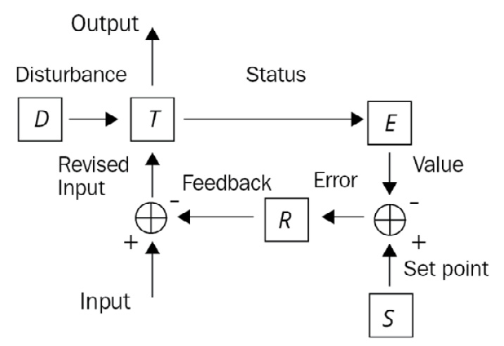
The behavior of a dynamical system is influenced by a feedback loop – a controller manipulates the system inputs to obtain the desired effect on the output. An error-controlled regulation is typically carried out with a proportional-integral-derivative (PID) controller, and as the name suggests, the signal is derived from a weighted sum, integral, and derivative of the error signal. The error, which is the difference between the actual and the desired output, is applied as feedback to the input. The standard terminology for a system is a process, and for a controlled variable is a process variable (PV), and the objective remains the reduction of the deviation error. Using a negative feedback loop, a measurement of PV (E in Figure 1.5) is deducted from a desired value S (set point or SP) to estimate an error (SP minus PV) in the system, which is used by a regulator R (Figure 1.5) to reduce the gap between the measured value and desired value. The error may be introduced into the system T as a disturbance D, as shown in the closed loop (Figure 1.5) of a controller.

Figure 1.5: Negative feedback controller
Control theory can be linear as well as non-linear. Linear control theory is applied to devices obeying the superposition principle, meaning the output is roughly proportional to the input. Such (close to ideal) systems are tractable by frequency domain mathematical techniques such as Laplace transform, Fourier transform, and the Nyquist stability criterion. Non-linear control theory, on the other hand, applies to real-world systems that do not obey the superposition principle. Such systems are often governed by non-linear differential equations and analyzed using numerical methods. Non-linear systems are studied numerically using simulating operations using a simulation language that mirrors the system processes. However, if solutions in the vicinity of a stable or equilibrium point are only of interest, non-linear control systems can be linearized into approximations using perturbation techniques.
Understanding the problem
Mathematical techniques are served in either the frequency domain or time domain for analyzing control systems. The state variables in a frequency domain, representing the system’s input, output, and feedback, are functions of frequency. The transfer function, system function, or network function is a mathematical model of the relationship between the input and output, on the basis of differential equations governing or describing the system. The input and transfer functions are converted from functions of time to functions of frequency by a mathematical transformation. In this domain, the differential equations are replaced by algebraic equations, which are simpler to solve. The state variables in a time domain are functions of time, and the system is described by one or more differential equations.
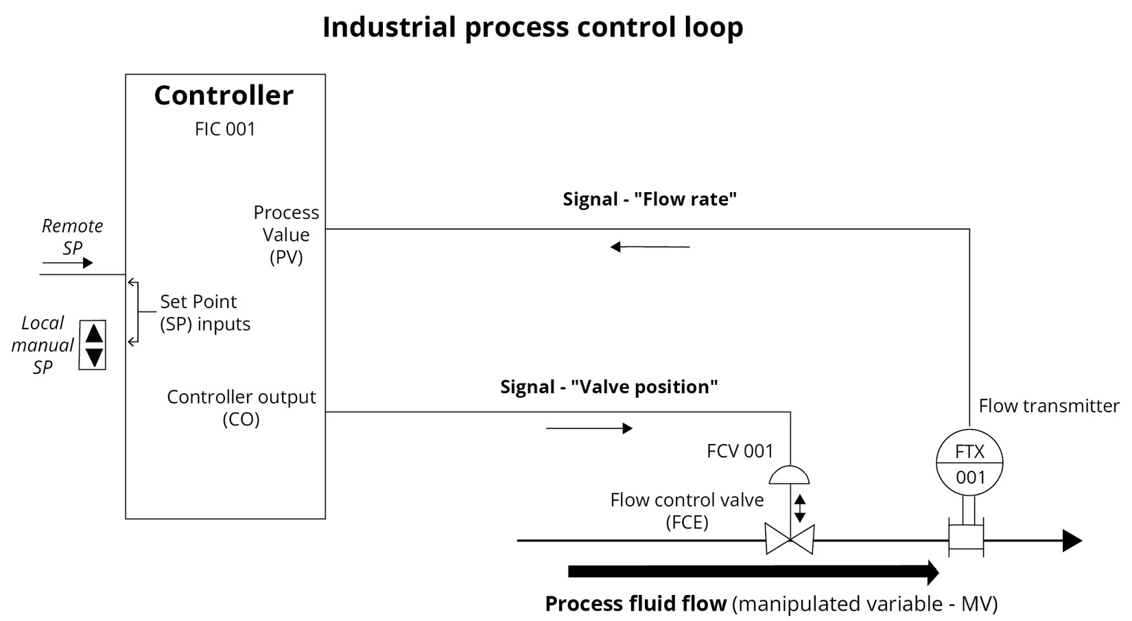
Time domain techniques are used to explore and analyze real non-linear systems because frequency domain techniques can only be used to study (ideal) linear systems. Although the equations for non-linear systems are difficult to solve, computer simulation methods have made their analyses commonplace. A critical application of the control loop is in industrial process control systems design, as shown in Figure 1.6.

Figure 1.6: Industrial control showing continuously modulated process flow
The building block of industrial processes is the control loop, which consists of all elements to measure and control a process value at a desired SP in the presence of perturbances. The controller may be an isolated piece of hardware or, within a large distributed control system, a programmable logic controller (PLC) system and SP inputs can be manually set or cascaded from another source. The green text in Figure 1.6 are tags that describe the function and identify a component and are unique (strings) within a plant representing the equipment components or elements. An associated sensor essentially captures the data of such tags.
Formulation of the problem
Modern control theory utilizes state-space methods (time-domain representation), unlike classical control theory, which uses transform methods (frequency-domain representation) such as the Laplace transform, which encodes all system information. In the state-space approach, a mathematical model is a set of first-order differential equations governing the related set of input, output, and state variables of the system. These variables are expressed as vectors, and the differential equations have a matrix format, which is more convenient to tackle. On the contrary, algebraic equations representing the behavior of a linear dynamical system are written in matrix form.
The state-space approach is not limited to linear systems and provides a convenient and compact way of modeling and analyzing mostly non-linear systems with multiple inputs and outputs. State space refers to a space whose axes are state variables, and the system state is expressed as a vector within that space.
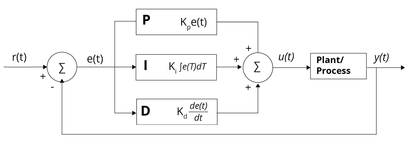
A plant or process is the part of the system that is controlled, and the controller (or simply filter) makes up the rest. Inputs to the process have an effect on the outputs, and the effect is measured with sensors and processed by the controller. The control signal is fed back to the input, thus closing the loop. Such a typical architecture is the PID controller, which is by and large the most used industrial design, shown in Figure 1.7. It calculates an error value e(t) continuously, the error being the difference between the desired SP and measured PV, and applies a correction on the basis of proportional, integral, and derivative terms.

Figure 1.7: u(t) is the control signal sent to the system, e(t) = r(t) – y(t) is the error
When such a process is monitored by multiple controllers, it becomes a distributed control system with a decentralized control loop. Decentralization is useful as it helps the control systems to operate over a large area while interaction happens through communication channels.
Some of the main control techniques extensively used in industries include adaptive control, hierarchical control, optimal control, robust control, and stochastic control. Apart from these, intelligent control uses artificial intelligence (AI) and ML approaches such as fuzzy logic, neural networks, and so on to control a dynamic system. Industry 4.0 is revolutionizing the way manufacturers are integrating AI into their operations and production facilities.


