The Minmax Algorithm
Suppose there is a game where a heuristic function can evaluate a game state from the perspective of the AI player. For instance, we used a specific evaluation for the tic-tac-toe exercise:
- +1,000 points for a move that won the game
- +100 points for a move preventing the opponent from winning the game
- +10 points for a move creating two in a row, column, or diagonal
- +1 point for a move creating one in a row, column, or diagonal
This static evaluation is straightforward to implement on any node. The problem is that as we go deep into the tree of all possible future states, we do not yet know what to do with these scores. This is where the Minmax algorithm comes into play.
Suppose we construct a tree with each possible move that could be performed by each player up to a certain depth. At the bottom of the tree, we evaluate each option. For the sake of simplicity, let's assume that we have a search tree that appears as follows:
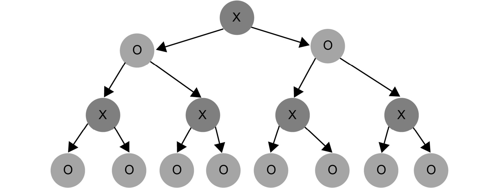
Figure 1.22: Example of a search tree up to a certain depth
The AI plays with X, and the player plays with O. A node with X means that it is X's turn to move. A node with O means it is O's turn to act.
Suppose there are all O leaves at the bottom of the tree, and we didn't compute any more values because of resource limitations. Our task is to evaluate the utility of the leaves:
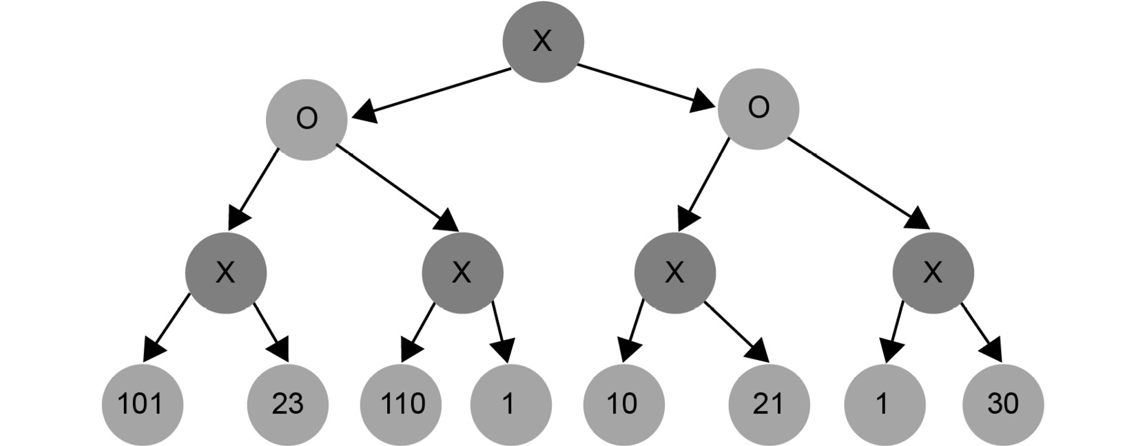
Figure 1.23: Example of a search tree with possible moves
We have to select the best possible move from our perspective because our goal is to maximize the utility of our move. This aspiration to maximize our gains represents the Max part in the Minmax algorithm:
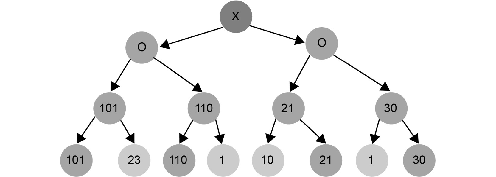
Figure 1.24: Example of a search tree with the best possible move
If we move one level higher, it is our opponent's turn to act. Our opponent picks the value that is the least beneficial to us. This is because our opponent's job is to minimize our chances of winning the game. This is the Min part of the Minmax algorithm:
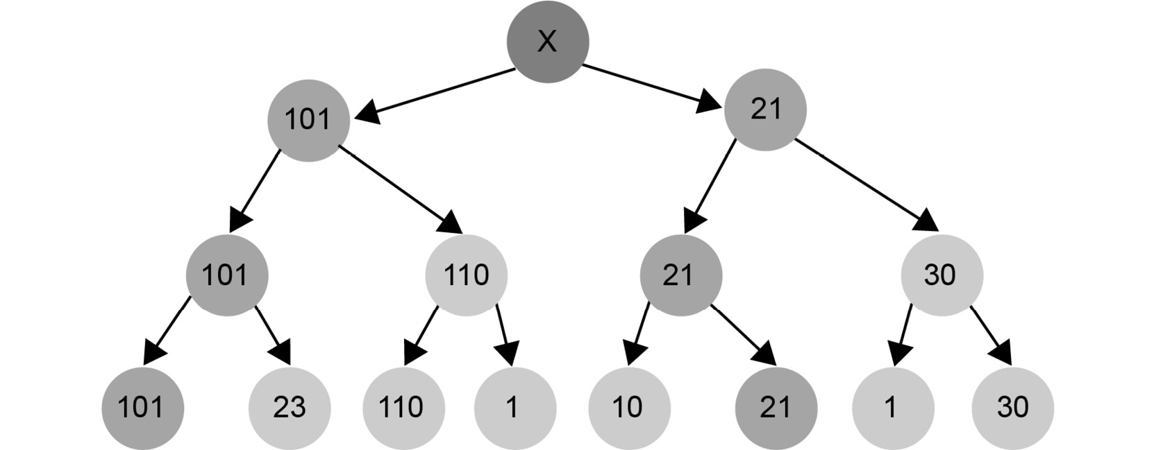
Figure 1.25: Minimizing the chances of winning the game
At the top, we can choose between a move with utility 101 and another move with utility 21. Since we are maximizing our value, we should pick 101:
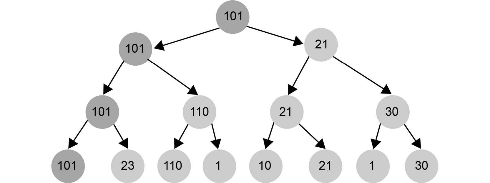
Figure 1.26: Maximizing the chances of winning the game
Let's see how we can implement this idea:
def min_max( state, depth, is_maximizing):
    if depth == 0 or is_end_state( state ):
        return utility( state )
    if is_maximizing:
        utility = 0
        for s in successors( state ):
            score = MinMax( s, depth - 1, false )
            utility = max( utility, score )
        return utility
    else:
        utility = infinity
        for s in successors( state ):
            score = MinMax( s, depth - 1, true )
            utility = min( utility, score )
        return utility
This is the Minmax algorithm. We evaluate the leaves from our perspective. Then, from the bottom up, we apply a recursive definition:
- Our opponent plays optimally by selecting the worst possible node from our perspective.
- We play optimally by selecting the best possible node from our perspective.
We need a few more things in order to understand the application of the Minmax algorithm on the tic-tac-toe game:
is_end_stateis a function that determines whether the state should be evaluated instead of digging deeper, either because the game has ended, or because the game is about to end using forced moves. Using our utility function, it is safe to say that as soon as we reach a score of 1,000 or higher, we have effectively won the game. Therefore,is_end_statecan simply check the score of a node and determine whether we need to dig deeper.- Although the
successorsfunction only depends on the state, it is practical to pass the information of whose turn it is to make a move. Therefore, do not hesitate to add an argument if needed; you do not have to follow the pseudo code. - We want to minimize our efforts in implementing the Minmax algorithm. For this reason, we will evaluate existing implementations of the algorithm. We will also simplify the duality of the description of the algorithm in the remainder of this section.
- The suggested utility function is quite accurate compared to the utility functions that we could be using in this algorithm. In general, the deeper we go, the less accurate our utility function has to be. For instance, if we could go nine steps deep into the tic-tac-toe game, all we would need to do is award 1 point for a win, 0 for a draw, and -1 point for a loss, given that, in nine steps, the board is complete, and we have all of the necessary information to make the evaluation. If we could only look four steps deep, this utility function would be completely useless at the start of the game because we need at least five steps to win the game.
- The Minmax algorithm could be optimized further by pruning the tree. Pruning is an act where we get rid of branches that do not contribute to the result. By eliminating unnecessary computations, we save precious resources that could be used to go deeper into the tree.
Optimizing the Minmax Algorithm with Alpha-Beta Pruning
The last consideration in the previous thought process primed us to explore possible optimizations by reducing the search space by focusing our attention on nodes that matter.
There are a few constellations of nodes in the tree where we can be sure that the evaluation of a subtree does not contribute to the end result. We will find, examine, and generalize these constellations to optimize the Minmax algorithm.
Let's examine pruning through the previous example of nodes:
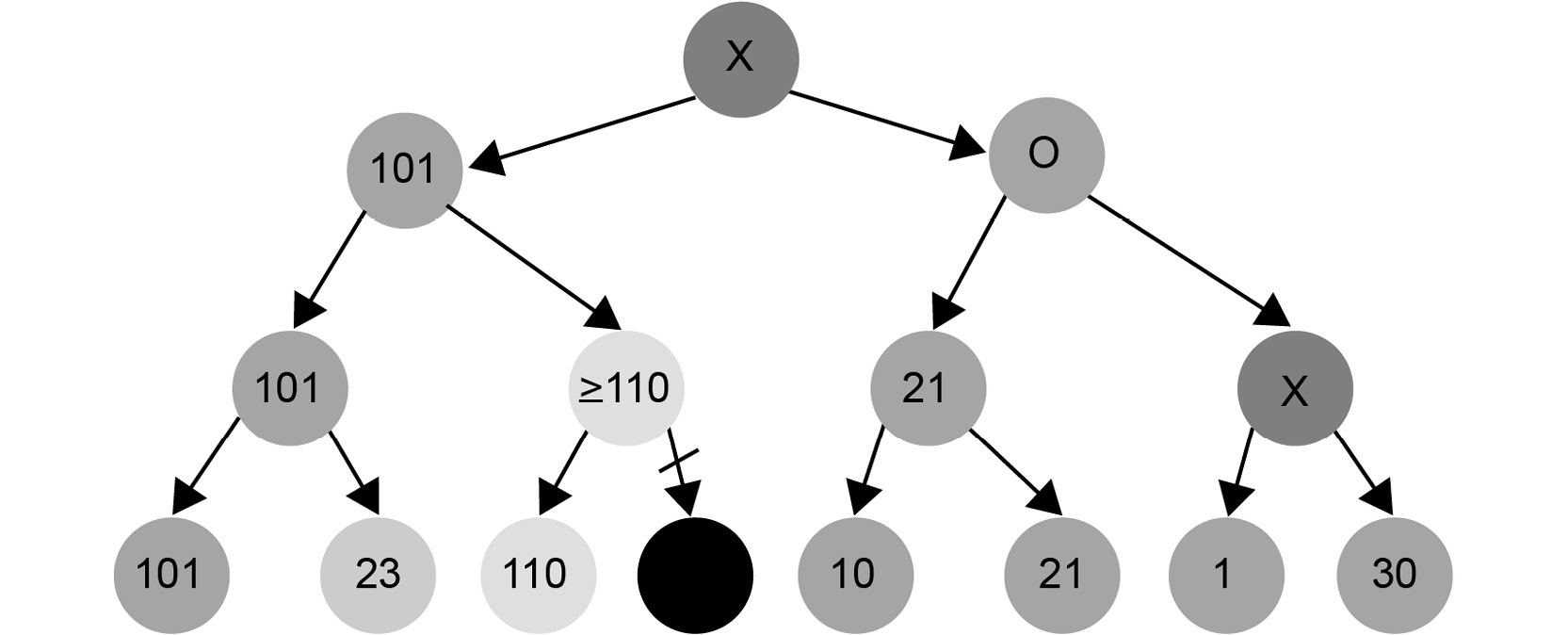
Figure 1.27: Search tree demonstrating pruning nodes
After computing the nodes with values 101, 23, and 110, we can conclude that two levels above, the value 101 will be chosen. Why?
- Suppose X <= 110. Here, the maximum of
110and X will be chosen, which is110, and X will be omitted. - Suppose X > 110. Here, the maximum of
110and X is X. One level above, the algorithm will choose the lowest value out of the two. The minimum of101and X will always be101, because X > 110. Therefore, X will be omitted a level above.
This is how we prune the tree.
On the right-hand side, suppose we computed branches 10 and 21. Their maximum is 21. The implication of computing these values is that we can omit the computation of nodes Y1, Y2, and Y3, and we know that the value of Y4 is less than or equal to 21. Why?
The minimum of 21 and Y3 is never greater than 21. Therefore, Y4 will never be greater than 21.
We can now choose between a node with utility 101 and another node with a maximal utility of 21. It is obvious that we have to choose the node with utility 101:
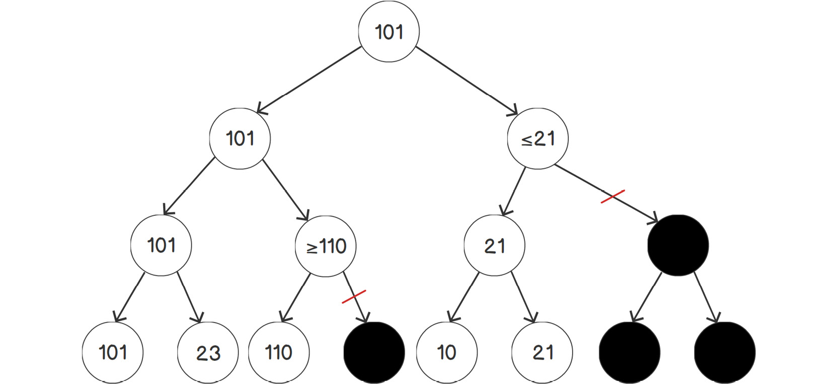
Figure 1.28: Example of pruning a tree
This is the idea behind alpha-beta pruning. We prune subtrees that we know are not going to be needed.
Let's see how we can implement alpha-beta pruning in the Minmax algorithm.
First, we will add an alpha and a beta argument to the argument list of Minmax:
def min_max(state, depth, is_maximizing, alpha, beta):
    if depth == 0 or is_end_state(state):
        return utility(state)
    if is_maximizing:
        utility = 0
        for s in successors(state):
            score = MinMax(s, depth - 1, false, alpha, beta)
            utility = max(utility, score)
            alpha = max(alpha, score)
            if beta <= alpha:
                break
        return utility
    else:
        utility = infinity
        for s in successors(state):
            score = MinMax(s, depth - 1, true, alpha, beta)
            utility = min(utility, score)
        return utility
In the preceding code snippet, we added the alpha and beta arguments to the MinMax function in order to calculate the new alpha score as being the maximum between alpha and beta in the maximizing branch.
Now, we need to do the same with the minimizing branch:
def min_max(state, depth, is_maximizing, alpha, beta):
    if depth == 0 or is_end_state( state ):
        return utility(state)
    if is_maximizing:
        utility = 0
        for s in successors(state):
            score = min_max(s, depth - 1, false, alpha, beta)
            utility = max(utility, score)
            alpha = max(alpha, score)
            if beta <= alpha: break
        return utility
    else:
        utility = infinity
        for s in successors(state):
            score = min_max(s, depth - 1, true, alpha, beta)
            utility = min(utility, score)
            beta = min(beta, score)
            if beta <= alpha: break
        return utility
In the preceding code snippet, we added the new beta score in the else branch, which is the minimum between alpha and beta in the minimizing branch.
We are done with the implementation. It is recommended that you mentally execute the algorithm on our example tree step by step to get a feel for the implementation.
One important piece is missing that has prevented us from doing the execution properly: the initial values for alpha and beta. Any number that is outside the possible range of utility values will do. We will use positive and negative infinity as initial values to call the Minmax algorithm:
alpha = infinity
beta = -infinity
In the next section, we will look at the DRYing technique while using the NegaMax algorithm.


