Search icon CANCEL
Subscription
0
Cart icon
Your Cart (0 item)
Close icon
You have no products in your basket yet
Save more on your purchases! discount-offer-chevron-icon
Savings automatically calculated. No voucher code required.
Arrow left icon
Explore Products
Best Sellers
New Releases
Books
Videos
Audiobooks
Learning Hub
Newsletter Hub
Free Learning
Arrow right icon
timer SALE ENDS IN
0 Days
:
00 Hours
:
00 Minutes
:
00 Seconds
Arrow up icon
GO TO TOP
Bayesian Analysis with Python

You're reading from   Bayesian Analysis with Python Unleash the power and flexibility of the Bayesian framework

Arrow left icon
Product type Paperback
Published in Nov 2016
Publisher Packt
ISBN-13 9781785883804
Length 282 pages
Edition 1st Edition
Languages
Arrow right icon
Author (1):
Arrow left icon
Osvaldo Martin Osvaldo Martin
Author Profile Icon Osvaldo Martin
Osvaldo Martin
Arrow right icon
View More author details
Toc

Table of Contents (10) Chapters Close

Preface 1. Thinking Probabilistically - A Bayesian Inference Primer FREE CHAPTER 2. Programming Probabilistically – A PyMC3 Primer 3. Juggling with Multi-Parametric and Hierarchical Models 4. Understanding and Predicting Data with Linear Regression Models 5. Classifying Outcomes with Logistic Regression 6. Model Comparison 7. Mixture Models 8. Gaussian Processes Index

Hierarchical linear regression

In the previous chapter, we learned the rudiments of hierarchical models. We can apply these concepts to linear regression and model several groups at the same time including estimations at the group level and estimations above the group level. As we saw, this is done by including hyperpriors.

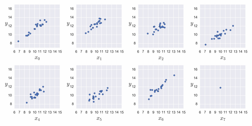
We are going to create eight related data groups, including one with just one data point:

N = 20
M = 8
idx = np.repeat(range(M-1), N)
idx = np.append(idx, 7)

alpha_real = np.random.normal(2.5, 0.5, size=M)
beta_real = np.random.beta(60, 10, size=M)
eps_real = np.random.normal(0, 0.5, size=len(idx))

y_m = np.zeros(len(idx))
x_m = np.random.normal(10, 1, len(idx))
y_m = alpha_real[idx] + beta_real[idx] * x_m  + eps_real

Our data looks like this:

j, k = 0, N
for i in range(M):
    plt.subplot(2,4,i+1)
    plt.scatter(x_m[j:k], y_m[j:k])
    plt.xlim(6, 15)
    plt.ylim(7, 17)
    j += N
    k += N
plt.tight_layout()
Hierarchical linear regression

Now we are going to center the data before feeding it to...

lock icon The rest of the chapter is locked
Register for a free Packt account to unlock a world of extra content!
A free Packt account unlocks extra newsletters, articles, discounted offers, and much more. Start advancing your knowledge today.
Unlock this book and the full library FREE for 7 days
Get unlimited access to 7000+ expert-authored eBooks and videos courses covering every tech area you can think of
Renews at $19.99/month. Cancel anytime
Banner background image