Estimating with decision tree regression
Decision tree regression is also called a regression tree. It is easy to understand a regression tree by comparing it with its sibling, the classification tree, which you are already familiar with. In this section, we will delve into employing decision tree algorithms for regression tasks.
Transitioning from classification trees to regression trees
In classification, a decision tree is constructed by recursive binary splitting and growing each node into left and right children. In each partition, it greedily searches for the most significant combination of features and its value as the optimal splitting point. The quality of separation is measured by the weighted purity of the labels of the two resulting children, specifically via Gini Impurity or Information Gain.
In regression, the tree construction process is almost identical to the classification one, with only two differences because the target becomes continuous:
- The quality of the splitting point is now measured by the weighted MSE of two children; the MSE of a child is equivalent to the variance of all target values, and the smaller the weighted MSE, the better the split
- The average value of targets in a terminal node becomes the leaf value, instead of the majority of labels in the classification tree
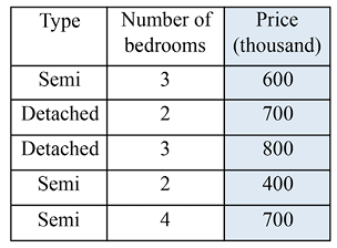
To make sure you understand regression trees, let’s work on a small house price estimation example using the house type and number of bedrooms:

Figure 5.8: Toy dataset of house prices
We first define the MSE and weighted MSE computation functions that will be used in our calculation:
>>> def mse(targets):
...     # When the set is empty
...     if targets.size == 0:
...         return 0
...     return np.var(targets)
Then, we define the weighted MSE after a split in a node:
>>> def weighted_mse(groups):
...     total = sum(len(group) for group in groups)
...     weighted_sum = 0.0
...     for group in groups:
...         weighted_sum += len(group) / float(total) * mse(group)
...     return weighted_sum
Test things out by executing the following commands:
>>> print(f'{mse(np.array([1, 2, 3])):.4f}')
0.6667
>>> print(f'{weighted_mse([np.array([1, 2, 3]), np.array([1, 2])]):.4f}')
0.5000
To build the house price regression tree, we first exhaust all possible feature and value pairs, and we compute the corresponding MSE:
MSE(type, semi) = weighted_mse([[600, 400, 700], [700, 800]]) = 10333
MSE(bedroom, 2) = weighted_mse([[700, 400], [600, 800, 700]]) = 13000
MSE(bedroom, 3) = weighted_mse([[600, 800], [700, 400, 700]]) = 16000
MSE(bedroom, 4) = weighted_mse([[700], [600, 700, 800, 400]]) = 17500
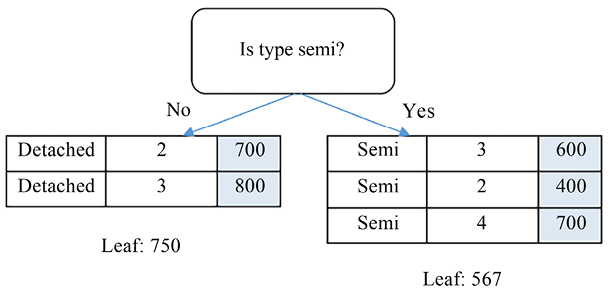
The lowest MSE is achieved with the type, semi pair, and the root node is then formed by this splitting point. The result of this partition is as follows:

Figure 5.9: Splitting using (type=semi)
If we are satisfied with a one-level regression tree, we can stop here by assigning both branches as leaf nodes, with the value as the average of the targets of the samples included. Alternatively, we can go further down the road by constructing the second level from the right branch (the left branch can’t be split further):
MSE(bedroom, 2) = weighted_mse([[], [600, 400, 700]]) = 15556
MSE(bedroom, 3) = weighted_mse([[400], [600, 700]]) = 1667
MSE(bedroom, 4) = weighted_mse([[400, 600], [700]]) = 6667
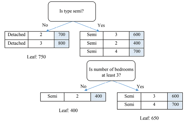
With the second splitting point specified by the bedroom, 3 pair (whether it has at least three bedrooms or not) with the lowest MSE, our tree becomes as shown in the following diagram:

Figure 5.10: Splitting using (bedroom>=3)
We can finish up the tree by assigning average values to both leaf nodes.
Implementing decision tree regression
Now that you’re clear about the regression tree construction process, it’s time for coding.
The node splitting utility function we will define in this section is identical to what we used in Chapter 3, Predicting Online Ad Click-Through with Tree-Based Algorithms, which separates samples in a node into left and right branches, based on a feature and value pair:
>>> def split_node(X, y, index, value):
...     x_index = X[:, index]
...     # if this feature is numerical
...     if type(X[0, index]) in [int, float]:
...         mask = x_index >= value
...     # if this feature is categorical
...     else:
...         mask = x_index == value
...     # split into left and right child
...     left = [X[~mask, :], y[~mask]]
...     right = [X[mask, :], y[mask]]
...     return left, right
Next, we define the greedy search function, trying out all the possible splits and returning the one with the least weighted MSE:
>>> def get_best_split(X, y):
...     """
...     Obtain the best splitting point and resulting children for the data set X, y
...     @return: {index: index of the feature, value: feature value, children: left and right children}
...     """
...     best_index, best_value, best_score, children =
                                     None, None, 1e10, None
...     for index in range(len(X[0])):
...         for value in np.sort(np.unique(X[:, index])):
...             groups = split_node(X, y, index, value)
...             impurity = weighted_mse(
                                [groups[0][1], groups[1][1]])
...             if impurity < best_score:
...                 best_index, best_value, best_score, children
                                   = index, value, impurity, groups
...     return {'index': best_index, 'value': best_value,
                'children': children}
The preceding selection and splitting process occurs recursively in each of the subsequent children. When a stopping criterion is met, the process at a node stops, and the mean value of the sample, targets, will be assigned to this terminal node:
>>> def get_leaf(targets):
...     # Obtain the leaf as the mean of the targets
...     return np.mean(targets)
And finally, here is the recursive function, split, that links it all together. It checks whether any stopping criteria are met and assigns the leaf node if so, proceeding with further separation otherwise:
>>> def split(node, max_depth, min_size, depth):
...     """
...     Split children of a node to construct new nodes or assign them terminals
...     @param node: dict, with children info
...     @param max_depth: maximal depth of the tree
...     @param min_size: minimal samples required to further split a child
...     @param depth: current depth of the node
...     """
...     left, right = node['children']
...     del (node['children'])
...     if left[1].size == 0:
...         node['right'] = get_leaf(right[1])
...         return
...     if right[1].size == 0:
...         node['left'] = get_leaf(left[1])
...         return
...     # Check if the current depth exceeds the maximal depth
...     if depth >= max_depth:
...         node['left'], node['right'] = get_leaf(
                             left[1]), get_leaf(right[1])
...         return
...     # Check if the left child has enough samples
...     if left[1].size <= min_size:
...         node['left'] = get_leaf(left[1])
...     else:
...         # It has enough samples, we further split it
...         result = get_best_split(left[0], left[1])
...         result_left, result_right = result['children']
...         if result_left[1].size == 0:
...             node['left'] = get_leaf(result_right[1])
...         elif result_right[1].size == 0:
...             node['left'] = get_leaf(result_left[1])
...         else:
...             node['left'] = result
...             split(node['left'], max_depth, min_size, depth + 1)
...     # Check if the right child has enough samples
...     if right[1].size <= min_size:
...         node['right'] = get_leaf(right[1])
...     else:
...         # It has enough samples, we further split it
...         result = get_best_split(right[0], right[1])
...         result_left, result_right = result['children']
...         if result_left[1].size == 0:
...             node['right'] = get_leaf(result_right[1])
...         elif result_right[1].size == 0:
...             node['right'] = get_leaf(result_left[1])
...         else:
...             node['right'] = result
...             split(node['right'], max_depth, min_size,
                       depth + 1)
The entry point of the regression tree construction is as follows:
>>> def train_tree(X_train, y_train, max_depth, min_size):
...     root = get_best_split(X_train, y_train)
...     split(root, max_depth, min_size, 1)
...     return root
Now, let’s test it with a hand-calculated example:
>>> X_train = np.array([['semi', 3],
...                     ['detached', 2],
...                     ['detached', 3],
...                     ['semi', 2],
...                     ['semi', 4]], dtype=object)
>>> y_train = np.array([600, 700, 800, 400, 700])
>>> tree = train_tree(X_train, y_train, 2, 2)
To verify that the trained tree is identical to what we constructed by hand, we write a function displaying the tree:
>>> CONDITION = {'numerical': {'yes': '>=', 'no': '<'},
...              'categorical': {'yes': 'is', 'no': 'is not'}}
>>> def visualize_tree(node, depth=0):
...     if isinstance(node, dict):
...         if type(node['value']) in [int, float]:
...             condition = CONDITION['numerical']
...         else:
...             condition = CONDITION['categorical']
...         print('{}|- X{} {} {}'.format(depth * ' ',
                  node['index'] + 1, condition['no'],
                  node['value']))
...         if 'left' in node:
...             visualize_tree(node['left'], depth + 1)
...         print('{}|- X{} {} {}'.format(depth * ' ',
                 node['index'] + 1, condition['yes'],
                 node['value']))
...         if 'right' in node:
...             visualize_tree(node['right'], depth + 1)
...     else:
...         print('{}[{}]'.format(depth * ' ', node))
>>> visualize_tree(tree)
|- X1 is not detached
  |- X2 < 3
    [400.0]
  |- X2 >= 3
    [650.0]
|- X1 is detached
  [750.0]
Now that you have a better understanding of the regression tree after implementing it from scratch, we can directly use the DecisionTreeRegressor package (https://scikit-learn.org/stable/modules/generated/sklearn.tree.DecisionTreeRegressor.html) from scikit-learn. Let’s apply it to an example of predicting California house prices. The dataset contains a median house value as the target variable, median income, housing median age, total rooms, total bedrooms, population, households, latitude, and longitude as features. It was obtained from the StatLib repository (https://www.dcc.fc.up.pt/~ltorgo/Regression/cal_housing.html) and can be directly loaded using the sklearn.datasets.fetch_california_housing function, as follows:
>>> housing = datasets.fetch_california_housing()
We take the last 10 samples for testing and the rest to train a DecisionTreeRegressor decision tree, as follows:
>>> num_test = 10 # the last 10 samples as testing set
>>> X_train = housing.data[:-num_test, :]
>>> y_train = housing.target[:-num_test]
>>> X_test = housing.data[-num_test:, :]
>>> y_test = housing.target[-num_test:]
>>> from sklearn.tree import DecisionTreeRegressor
>>> regressor = DecisionTreeRegressor(max_depth=10,
                                      min_samples_split=3,
                                      random_state=42)
>>> regressor.fit(X_train, y_train)
We then apply the trained decision tree to the test set:
>>> predictions = regressor.predict(X_test)
>>> print(predictions)
[1.29568298 1.29568298 1.29568298 1.11946842 1.29568298 0.66193704 0.82554167 0.8546936  0.8546936  0.8546936 ]
Compare predictions with the ground truth, as follows:
>>> print(y_test)
[1.12  1.072 1.156 0.983 1.168 0.781 0.771 0.923 0.847 0.894]
We see the predictions are quite accurate.
We have implemented a regression tree in this section. Is there an ensemble version of the regression tree? Let’s see next.


