Putting data on x and y axes
Cube space in SSAS is multi-dimensional. MDX allows you to display results on axes from 0, 1, and 2 up to 128. The first five axes have aliases: COLUMNS, ROWS, PAGES, SECTIONS, and CHAPTERS. However, the frontend tools such as SQL Server Management Studio (SSMS) or other application that you can use for writing and executing MDX queries only have two axes, x and y axis, or COLUMNS and ROWS.
As a result, we have two tasks to do when trying to fit the multi-dimensional data onto the limited axes in our frontend tool:
We must always explicitly specify a display axis for all elements in the SELECT list. We can use aliases for the first five axes: COLUMNS, ROWS, PAGES, SECTIONS, and CHAPTERS. We are also allowed to use integers,
0,1,2,3, and so on. But we are not allowed to skip axes. For example, the first axis must be COLUMNS (or0). ROWS (or1) cannot be specified, unless COLUMNS (or0) has been specified first.Since we only have two display axes to show our data, we must be able to "combine" multiple hierarchies into one query axis. In MDX and other query language terms, we call it "cross join".
It's fair to say that your job of writing the MDX queries is mostly trying to figure out how to project multi-dimensional data onto only two axes, namely, x and y. We will start by putting only one hierarchy on COLUMNS, and one on ROWS. Then we will use the CROSSJOIN function to "combine" more than one hierarchy into COLUMNS and ROWS.
Getting ready
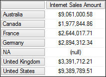
Making a two by eight table below in a spreadsheet is quite simple. Writing a MDX query to do that can also be very simple. Putting data on the x and y axes is a matter of finding the right expressions for each axis.
|
Internet Sales Amount | |
|---|---|
|
Australia |
$9,061,000.58 |
|
Canada |
$1,977,844.86 |
|
France |
$2,644,017.71 |
|
Germany |
$2,894,312.34 |
|
NA |
(null) |
|
United Kingdom |
$3,391,712.21 |
|
United States |
$9,389,789.51 |
All we need are three things from our cube:
The name of the cube
The correct expression for the Internet Sales Amount, so we can put it on the columns
The correct expression of the sales territory, so we can put it on the rows
Once, we have the preceding three things, we are ready to plug them into the following MDX query, and the cube will give us back the two by eight table:
SELECT
   [The Sales Expression] ON COLUMNS,
   [The Territory Expression] ON ROWS
FROM
   [The Cube Name]
The MDX engine will understand it perfectly, if we replace columns by 0 and rows by 1. Throughout this book, we will use the number 0 for columns that is the x axis, and 1 for rows that is the y axis.
How to do it…
We are going to use the Adventure Works 2012 Multidimensional Analysis Service database enterprise edition in our cookbook. If you open the Adventure Works cube, and hover your cursor over the measure Internet Sales Amount, you will see the fully qualified expression, [Measures].[Internet Sales Amount]. This is a long expression. Drag-and-drop in SQL Server Management Studio works perfectly for us in this situation.
Tip
Long expression is a fact of life in MDX. Although the case does not matter, correct spelling is required and fully qualified and unique expressions are recommended for MDX queries to work properly.
Follow these two steps to open the Query Editor in SSMS:
Start SQL Server Management Studio (SSMS) and connect to your SQL Server Analysis Services (SSAS) 2012 instance (
localhostorservername\instancename).Click on the target database Adventure Works DW 2012, and then right-click on the New Query button.
Follow these steps to save the time spent for typing the long expressions:
Put your cursor on measure Internet Sales Amount, and drag-and-drop it onto
AXIS(0).To get the proper expression for the sales territory, put your cursor over the Sales Territory Country under the Sales Territory | Sales Territory Country. Again, this is a long expression. Drag-and-drop it onto
AXIS(1).For the name of the cube, the drag-and-drop should work too. Just point your cursor to the cube name, and drag-and-drop it in your
FROMclause.
This should be your final query:
SELECT
   [Measures].[Internet Sales Amount] ON 0,
   [Sales Territory].[Sales Territory Country].[Sales Territory Country] ON 1
FROM
   [Adventure Works]
Tip
Downloading the example code
You can download the example code files for all Packt books you have purchased from your account at http://www.packtpub.com. If you purchased this book elsewhere, you can visit http://www.packtpub.com/support and register to have the files e-mailed directly to you.
When you execute the query, you should get a two by eight table, same as the following screenshot:

How it works…
We have chosen to put Internet Sales Amount on the Axis(0), and all members of Sales Territory Country on the Axis(1). We have fully qualified the measure with the special dimension [Measures], and the sales territory members with dimension [Sales Territory] and hierarchy [Sales Territory Country].
You might have expected an aggregate function such as SUM somewhere in the query. We do not need to have any aggregate function here because the cube understands that when we ask for the sales amount for Canada, we would expect the sales amount to come from all the provinces and territories in Canada.
There's more…
SSAS cubes are perfectly capable of storing data in more than two dimensions. In MDX, we can use the technique called "cross join" to "combine" multiple hierarchies into one query axis.
Putting more hierarchies on x and y axes with cross join
In MDX query, we can specify how multi-dimensions from our SSAS cube layout onto only two x and y axes. Cross joining allows us in both SQL and MDX to get every possible combination of two lists.
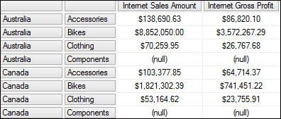
We wish to write an MDX query to produce the following table. On the columns axis, we want to see both Internet Sales Amount and Internet Gross Profit. On the rows axis, we want to see all the sales territory countries, and all the products sold in each country.
|
Internet Sales Amount |
Internet Gross Profit | ||
|---|---|---|---|
|
Australia |
Accessories |
$138,690.63 |
$86,820.10 |
|
Australia |
Bikes |
$8,852,050.00 |
$3,572,267.29 |
|
Australia |
Clothing |
$70,259.95 |
$26,767.68 |
|
Australia |
Components |
(null) |
(null) |
|
Canada |
Accessories |
$103,377.85 |
$64,714.37 |
|
Canada |
Bikes |
$1,821,302.39 |
$741,451.22 |
|
Canada |
Clothing |
$53,164.62 |
$23,755.91 |
|
Canada |
Components |
(null) |
(null) |
This query lays two measures on columns (from the same dimension and hierarchy [Measures]), and two different hierarchies [Sales Territory Country] and [Product Categories] on rows.
SELECT
   { [Measures].[Internet Sales Amount],
     [Measures].[Internet Gross Profit]
   } ON 0,
   { [Sales Territory].[Sales Territory Country].[Sales Territory
     Country] *
     [Product].[Product Categories].[Category]
   } ON 1
FROM
   [Adventure Works]
To return the cross product of two sets, we can use either of the following two syntaxes:
Standard syntax: Crossjoin(Set_Expression1, Set_Expression2)
Alternate syntax: Set_Expression1 * Set_Expression2
We have chosen to use the alternate syntax for its convenience. The result from the previous query is shown as follows:


