Overview of Pandas
In short, Pandas is our main module for working with data. The module is brimming with useful functions and tools, but let's get down to the basics first. The greatest tool of Pandas is its data structure, which is known as a DataFrame. In short, a DataFrame is a two-dimensional data structure with a good interface and great codability.
The DataFrame makes itself useful to you right off the bat. The moment you read a data source using Pandas, the data is restructured and shown to you as a DataFrame. Let's give it a try.
We will use the famous adult dataset (adult.csv) to practice and learn the different functionalities of Pandas. Refer to the following screenshot, which shows the importing of Pandas and then reading and showing the dataset. In this code, .head() requests that only the top five rows of data are output. The .tail() code could do the same for the bottom five rows of the data.
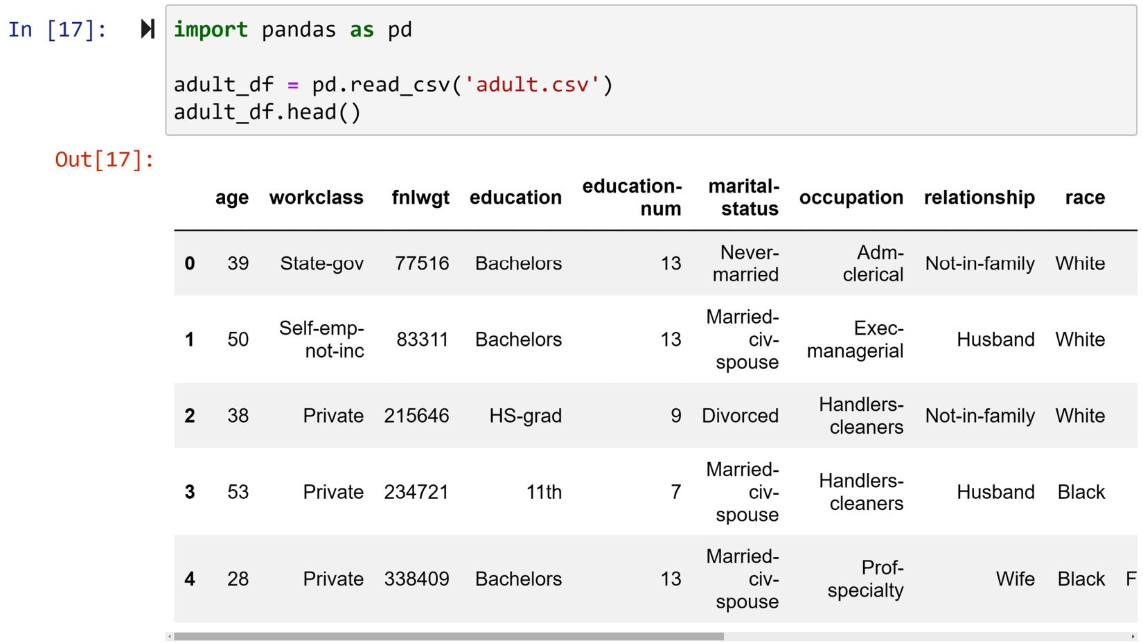
Figure 1.12 – Reading the adult.csv file using pd.read_csv() and showing its first five rows
The adult dataset has six continuous and eight categorical attributes. Due to print limitations, I have only been able to include some parts of the data; however, if you pay attention to Figure 1.12, the output comes with a scroll bar at the bottom that you can scroll to see the rest of the attributes. Give this code a try and study its attributes. As you will see, all of the attributes in this dataset are self-explanatory, apart from fnlwgt. The title is short for final weight and it is calculated by the Census Bureau to represent the ratio of the population that each row represents.
Good practice advice
It is good practice to always get to know the dataset you are about to work on. This process always starts with making sure you understand each attribute, the way I just did now. If you have just received a dataset and you don't know what each attribute is, ask. Trust me, you will look more like a pro than not.
There are other steps to get to know a dataset. I will mention them all here and you will learn how to do them by the end of this chapter.
Step one: Understand each attribute as I just explained.
Step two: Check the shape of the dataset. How many rows and columns does the dataset have? This one is easy. For instance, just try adult_df.shape and review the result.
Step three: Check whether the data has any missing values.
Step four: Calculate summarizing values for numerical attributes such as mean, median, and standard deviation, and compute all the possible values for categorical attributes.
Step five: Visualize the attributes. For numerical attributes, use a histogram or a boxplot, and for categorical ones, use a bar chart.
As you just saw, before you know it, you are enjoying the benefits of a Pandas DataFrame. So it is important to better understand the structure of a DataFrame. Simply put, a DataFrame is a collection of series. A series is another Pandas data structure that does not get as much credit, but is useful all the same, if not more so.
To understand this better, try to call some of the columns of the adult dataset. Each column is a property of a DataFrame, so to access it, all you need to do is to use .ColumnName after the DataFrame. For instance, try running adult_df.age to see the column age. Try running all of the columns and study them, and if you come across errors for some of them, do not worry about it; we will address them soon if you continue reading. The following screenshot shows how you can confirm what was just described for the adult dataset:

Figure 1.13 – Checking the type of adult_df and adult_df.age
It gets more exciting. Not only is each attribute a series, but each row is also a series. To access each row of a DataFrame, you need to use .loc[] after the DataFrame. What comes between the brackets is the index of each row. Go back and study the output of df_adult.head() in Figure 1.12 and you will see that each row is represented by an index. The indices do not have to be numerical and we will see how indices of a Pandas DataFrame can be adjusted, but when reading data using pd.read_csv() with default properties, numerical indices will be assigned. So give it a try and access some of the rows and study them. For instance, you can access the second row by running adult_df.loc[1]. After running a few of them, run type(adult_df.loc[1]) to confirm that each row is a series.
When accessed separately, each column or row of a DataFrame is a series. The only difference between a column series and a row series is that the index of a column series is the index of the DataFrame, and the index of a row series is the column names. Study the following screenshot, which compares the index of the first row of adult_df and the index of the first column of adult_df:

Figure 1.14 – Investigating the index for a column series and a row series
Now that we have been introduced to Pandas data structures, next we will cover how we can access the values that are presented in them.
Pandas data access
One of the greatest advantages of both Pandas series and DataFrames is the excellent access they afford us. Let's start with DataFrames, and then we will move on to series as there are lots of commonalities between the two.
Pandas DataFrame access
As DataFrames are two-dimensional, this section first addresses how to access rows, and then columns. The end part of the section will address how to access each value.
DataFrame access rows
The only two keywords you will ever need to access the rows of a DataFrame are .loc[] and .iloc[]. To understand the difference between them, you need to know that each Pandas series or DataFrame carries two types of indices: default indices or assigned indices. The default indices are the integer numbers that are automatically assigned to your dataset upon reading. However, Pandas allows you to update them. The function that you can use to do so is .set_index(). For instance, we would like to make sure all of the indices in adult_df have five digits, so instead of indices between 0 and 32651 (run len(adult_df) to see that this is the number of rows adult_df has), we want indices to be from 10000 to 42651. The following screenshot uses np.arange() and .set_index() to do this. In this code, inplace=True indicates to the .set_index() function that you want the change to be applied to the DataFrame itself.
Why is it that when inplace=True is incorporated, there is no output, and when it is included, Jupyter Notebook shows the updated DataFrame?
The answer is that the .set_index() function, by default, outputs a new DataFrame that has the requested index unless inplace=True is specified, which requests the change to be applied to the original DataFrame.
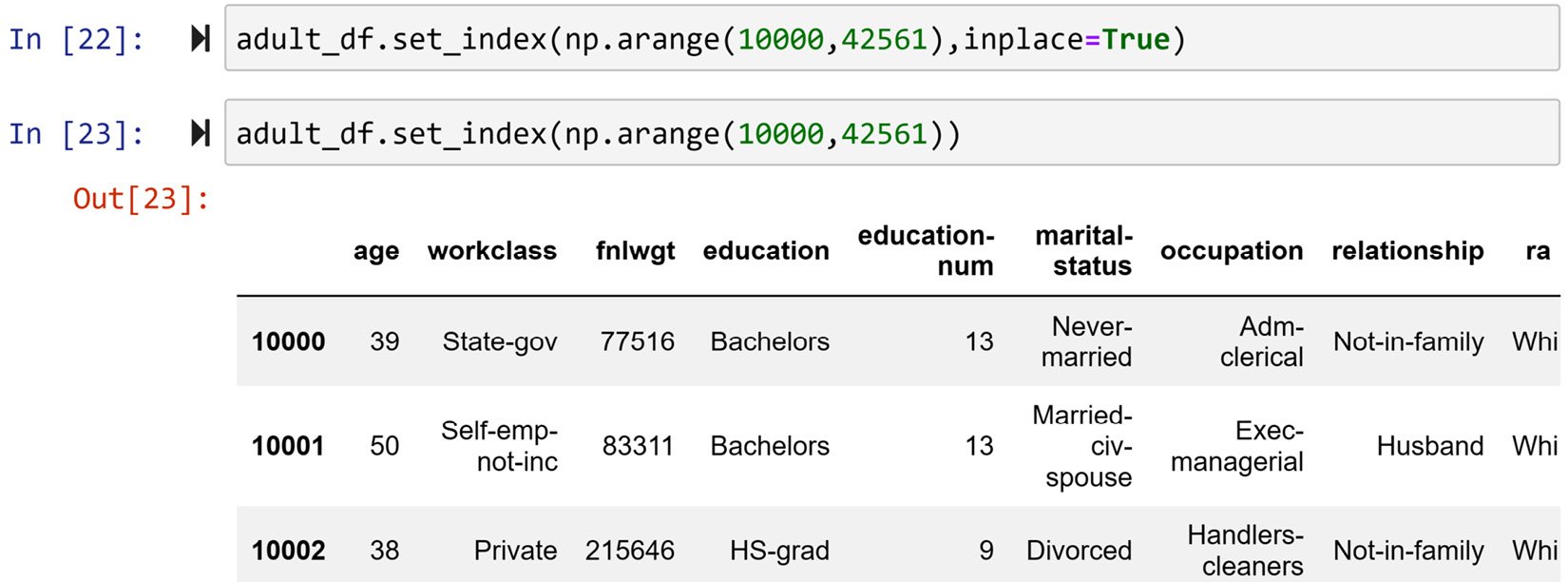
Figure 1.15 – Updating the index of adult_df as described
Now, each row of the DataFrame can be accessed by specifying the index in between the brackets of .loc[]. For instance, running adult_df.loc[10001] will give you the second row. This is how you would always access the DataFrame using the assigned indices. If you started missing the default indices, as you often do when you go about preprocessing your data, Pandas has you covered.
You can use .iloc[] to access the data using the default integer indices. For instance, running adult_df.iloc[1] will also return the second row. In other words, Pandas will change the index to your liking, but behind the scenes, it will also keep its integer default index and also lets you use it if you so wish.
DataFrame access columns
As there are two ways to access each row, there are also two ways to access each column. The easier and better way to access your columns is to know that each column is coded to be a property of a DataFrame. So, you can access each column by using .ColumnName. For instance, run adult_df.age, adult_df.occupation, and so on to see how easy it is to access the columns in this way.
If you happened to run adult_df.education-number, you have already seen that this gives you an error. If you haven't, go ahead and do so to study the error. Why does this error happen?

Figure 1.16 – Running adult_df.education-number and its error
If you study the error message, it is prompting that 'num' is not defined. That is true; we do not have anything named 'num'. That is the key to use this error to answer my question.
Python deciphers dashes as subtraction operators unless presented inside a quotation. So it all comes down to this. Because of the way this variable is named, you cannot use the .ColumnName method to access the variable. You either need to change the name of the variable or use the second method to access the columns.
The second method passes the name as a string, or, in other words, inside a quotation. Try running adult_df['education-num'] and this time you will not get an error.
Good practice advice
If you are new to programming, one of the pieces of advice that I have for you is not to be intimidated by errors, and not only that, welcome errors with open arms because they are an excellent opportunity to learn. I just used an error to teach you something.
DataFrame access values
Imagine you want to access the education value for the third row of adult_df. There are so many ways you can go about this. You can start from the column and once you get a column series, access the value, or you can go from the row, and once you get a row series, access the value. Study the following screenshot; the first three chunks of code show different possibilities of doing that. However, my favorite way to access the values is to use .at[], shown in the last chunk.
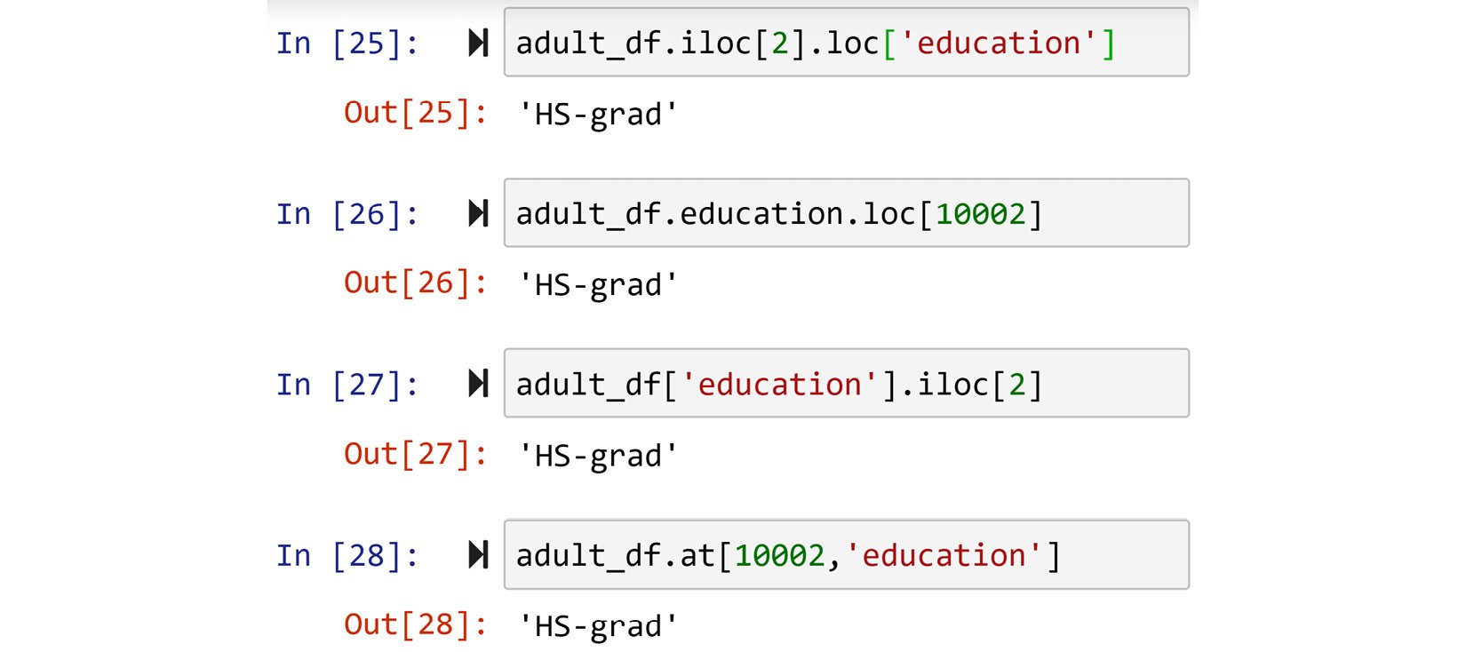
Figure 1.17 – Four different methods of accessing the records of a Pandas DataFrame
Accessing values with .at[] is my favorite for two reasons. First, it is much neater and more straightforward. Second, you can treat the DataFrame like a matrix as it is one, at least visually.
Pandas series access
Access to the values of series is very similar to that of DataFrames, just simpler. You can access the values of a series using all of the methods mentioned for DataFrames, except for .at[]. You can see all of the possibilities in the following screenshot. If you were to try the last line of the second chunk of code, Python would generate a syntax error as numbers cannot be the name of programming objects. To use this method, you have to make sure that the series indices are of the string type.
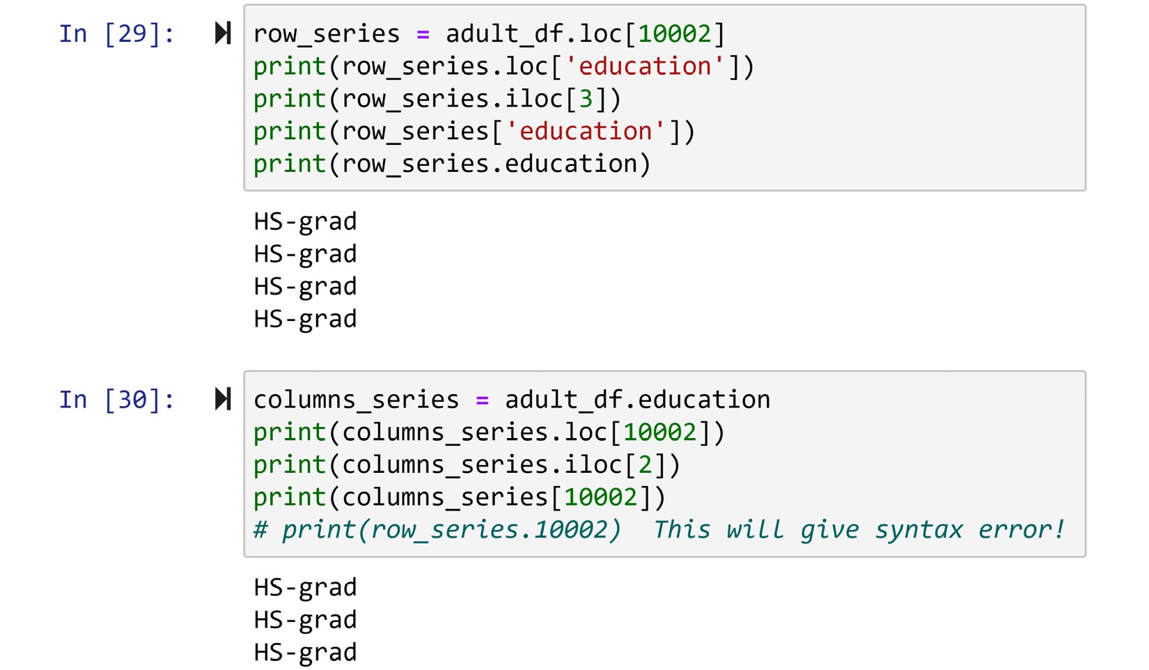
Figure 1.18 – Different methods of accessing the values of a Pandas series
Slicing
Slicing applies to both NumPy and Pandas; however, since this is a book about data preprocessing, we will use it more often with a Pandas DataFrame. Let's begin by slicing NumPy arrays to understand slicing and then apply it to a Pandas DataFrame.
Slicing a NumPy array
We slice a NumPy array when we need access to more than one value of the data. For instance, consider the code in the following screenshot:
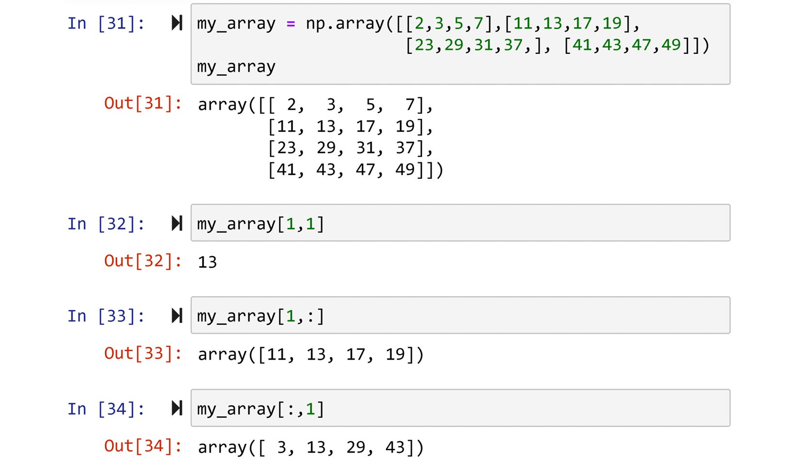
Figure 1.19 – Examples of slicing NumPy arrays
Here, my_array, which is a 4 x 4 matrix, has been sliced in different ways. The second chunk of code is not slicing; as you can see, only one value is accessed. What separates normal access from slicing access is the presence of a colon (:) in any of the index inputs. For instance, a colon in the third chunk of code means you are requesting all of the columns, and the output includes all of the columns, but since only the second row (index 1) is specified, the entirety of the second row is output. The fourth chunk of code is the opposite; one column is specified and the whole rows are requested, so the entirety of the second column is output.
You can also use a colon (:) to only specify access from a certain index to another one. For instance, in the second chunk of the following code, while all the columns are requested, only the second to fourth rows (1:3) are requested. The third chunk of code shows that both columns and rows can be sliced at the same time. Finally, the last chunk of code shows that you can pass a list of indices that you want to include in your slice.
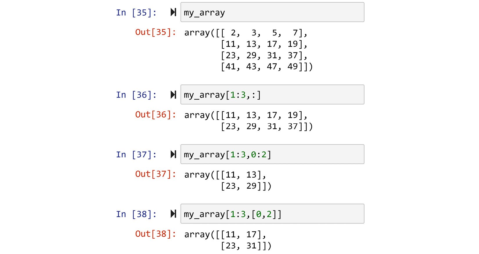
Figure 1.20 – More complex examples of slicing
Slicing a Pandas DataFrame
Just like NumPy arrays, Pandas DataFrames can also be sliced both on the columns and rows. However, the slicing function can only be done inside either .loc[] or .iloc[]. The access method, .at[], and the other ways of accessing data do not support slicing. For instance, the following code slices adult_df to show all of the rows, but only the columns from education to occupation. Running adult_df.iloc[:,3:6] will result in the same output.

Figure 1.21 – Example of slicing a Pandas DataFrame
You want to become comfortable with slicing a Pandas DataFrame. It is a very useful way to access your data. See the following example, which showcases one practical way in which you could use slicing.
Practical example of slicing
Run adult_df.sort_values('education-num'). You will see this code sort the DataFrame based on the education-num column. In Jupyter Notebook output, you only see the first five and the last five rows of this sorting. Slice the output of the rows from across the DataFrame instead of just from the beginning and the end.
The following screenshot shows how slicing the DataFrame can make this happen:
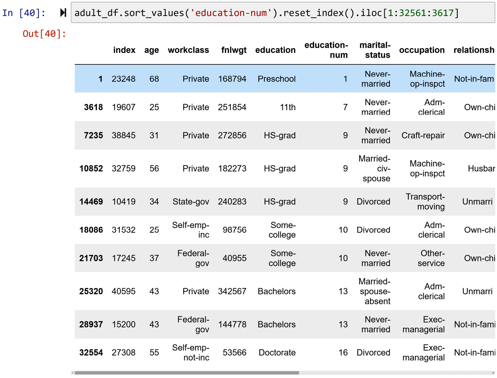
Figure 1.22 – Solution to the practical example of slicing a Pandas DataFrame
Let's go over this code step by step:
- The first part,
.sort_values('education-num'), as mentioned, sorts the DataFrame byeducation-num. I hope you have given this a try before reading on. Pay attention to the indices of the sortedadult_df. They look jumbled up, as they should. The reason is that the DataFrame is now sorted by another column. - If we want to have a new index that matches this new order, we can use
.reset_index(), as it has been used in the preceding screenshot. Go ahead and give this a try as well. Runadult_df.sort_values('education-num').reset_index(). You will see that the old index is presented as a new column and that the new index looks as ordered as any newly read dataset. - Adding
.iloc[1:32561:3617]achieves what this example is asking. This specific slice requests the first row and every 3,617th row after that until the end of the DataFrame. The number 32561 is the number of rows inadult_df(runlen(adult_df)), and 3617 is the quotient of the division of 32561 by 9. This division calculates the equal jumps that take us from row one to nearly the end ofadult_df. Pay attention if the division of 32561 by 9 didn't have a remainder; the code would take you all the way to the end of the DataFrame.Good practice advice
Being able to slice DataFrames this way is advantageous in the initial stages of getting to know a dataset. One of the disadvantages of data manipulations using programming instead of spreadsheet software such as Excel is that you cannot scroll through the data as you would in Excel. However, slicing the data this way can allow you to somehow mitigate this shortcoming.
Now that we have learned how to access and slice a dataset, we need to learn how to filter the data based on our needs. To do that, next we will learn about Boolean masking, which is a powerful filtering technique.
Boolean masking for filtering a DataFrame
One of the simplest and yet most powerful tools of working with data is Boolean masking. When you want to filter a DataFrame using a Boolean mask, you need a one-dimensional collection of Boolean values (True or False) that has as many Boolean values as the number of rows of DataFrames you want to filter.
The following screenshot shows an example of Boolean masking:

Figure 1.23 – Example of Boolean masking
The code portrays Boolean masking in three steps:
- The code first creates the Pandas series
twopowers_sr, which contains the values of 2 to the power of 0 through 10 (20, 21, 22, ..., 210). - Then, a Boolean mask is set up. Pay attention as
twopowers_srhas 11 numerical values, whileBMalso has 11 Boolean values. From now on in this book, every time you seeBM, you can safely assume it stands for Boolean mask. - The last line of code filters the series using the mask.
The way a Boolean mask works is straightforward. If the counterpart of the numerical value from twopowers_sr in the Boolean mask (BM) is False, the mask blocks the number, and if it is True, the mask lets it through. Check whether that has been the case regarding the output of the preceding code. This is shown in the following figure:

Figure 1.24 – Depiction of Boolean masking
What is great about Pandas is that you can use the DataFrame or series themselves to create useful Boolean masks. You can use any of the mathematical comparison operators to do this. For instance, the following screenshot first creates a Boolean mask that would only include True for numbers greater than or equal to 500. Then, the Boolean mask is applied to twopowers_sr to filter out the numbers in two ways.
Both of these ways are legitimate, correct, and they work. On the first one, you still give the Boolean mask a name. We use the name BM to do this as mentioned earlier. Then, we use BM to apply the Boolean mask. On the second one, you create and use the Boolean mask on the fly, as programmers say. That means you do everything in one line of code. I use the first one more often than not as I believe it makes the code more readable.
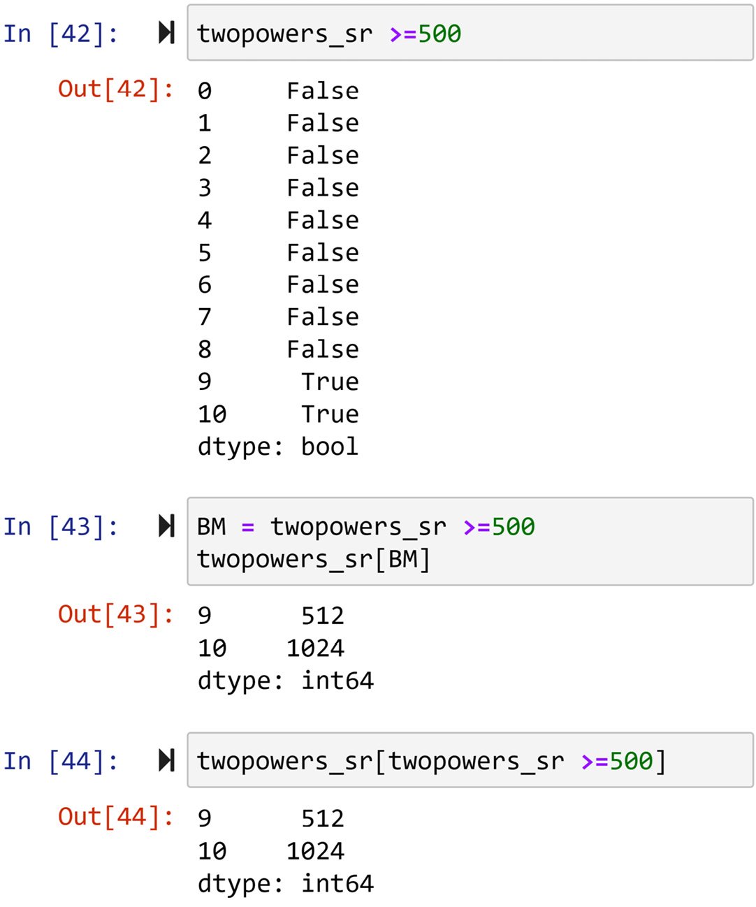
Figure 1.25 – Example of Boolean masking to filter data
You might be asking from the preceding code, so what if we can filter the data using Boolean masking? That is a legitimate question. Boolean masks come into their own when you use them on DataFrames for analytics. The following two examples will clarify this for you.
Analytic example 1 that uses Boolean masking
We are interested in calculating the mean and median age of people with preschool education in adult_df.
This can be easily done using Boolean masking. The following screenshot first creates BM using the series adult_df.education.

Figure 1.26 – Solution to the preceding example
Since the BM series has as many elements as the adult_df DataFrame (why?), BM can be applied to filter it. Once the DataFrame is filtered using adult_df[BM], it only contains rows that their education is 'Preschool'. So now you can easily use np.mean() and np.median() to calculate the mean and median of age for these filtered rows.
Analytic example 2 that uses Boolean masking
We are interested in comparing the Capital Gain of individuals with less than 10 years' education with individuals with more than 10 years' education.

Figure 1.27 – Solution to the preceding example
Again, Boolean masks can help us immensely here. Two of them, BM1 and BM2, are first created based on what we are interested in calculating. Then, two calculations and reports show the mean of the capital gain for people with more than, and less than, 10 years of education.
Pandas functions for exploring a DataFrame
When you compare spreadsheet software such as Excel with coding, one of the stark disadvantages of coding is that you cannot create as tangible a relationship with your data as you would with Excel. That is a fair comparison as Excel lets you scroll up and down on your data and so allows you to get to know it. While coding does not grant you this privilege, Pandas has a handful of useful functions that help you to familiarize yourself with the data.
Getting to know a dataset has two aspects. The first is to get to know the structure of the data, such as the number of rows, columns, and the name of columns. The second one is to get to know the values under each column. So we first cover getting to know the structure of the dataset and then we will focus on the values under each column.
Getting to know the structure of a dataset
You can use three useful properties of a Pandas Dataframe to study the structure of a dataset. These are .shape, .columns, and .info(). In the following sections, we will go over them one by one.
The .shape property
.shape is the property of any Pandas DataFrame. It tells you how many rows and columns the DataFrame has. So, once you apply this to adult_df, as executed by the code in the following screenshot, you can see that the DataFrame has 32,561 rows and 15 columns:

Figure 1.28 – Example of using the .shape property of a DataFrame to get to know the dataset
The .columns property
.columns allows you to see and edit the column names in your DataFrame. In the following code, you can see that adult_df.columns resulted in the output of all the column names of adult_df. Of course, you could have scrolled to see all of the columns when you read the dataset; however, this is not possible when the data has more than 20 columns.

Figure 1.29 – Example of using the .columns property of a DataFrame to get to know the dataset
Furthermore, .columns can be used to update the columns' names. This has been shown in the following screenshot. After running the following code, you can safely use adult_df.education_num to access the relevant attribute. We just change the attribute name from 'education-num' to 'education_num' and now the attribute can be accessed using the .columnName method. Refer to Figure 1.16, which showed the error you'd get if you were to run adult_df.education-num.

Figure 1.30 – Example of updating the column titles of a DataFrame
The .info() function
This function provides information about both the shape and the columns of the DataFrame. If you run adult_df.info(), you will see other information, such as the number of non-null values and also the type of data under each column that will be reported.
Getting to know the values of a dataset
The functions that Pandas has to get to know the numerical columns are different than those of categorical columns. The difference between numerical and categorical columns is that categorical columns are not represented by numbers or, more accurately, do not carry numerical information.
To get to know numerical columns, the .describe(), .plot.hist(), and .plot.box() functions are very useful. On the other hand, the .unique() and .value_counts() functions are instrumental for categorical columns. We will cover these one by one.
The .describe() function
This function outputs many useful statistical metrics that are meant to summarize data for each column. These metrics include Count, Mean, Standard Deviation (std), Minimum (min), first quartile (25%), second quartile (50%) or median, third quartile (75%), and Maximum (max). The following screenshot shows the execution of the function for adult_df and its output:
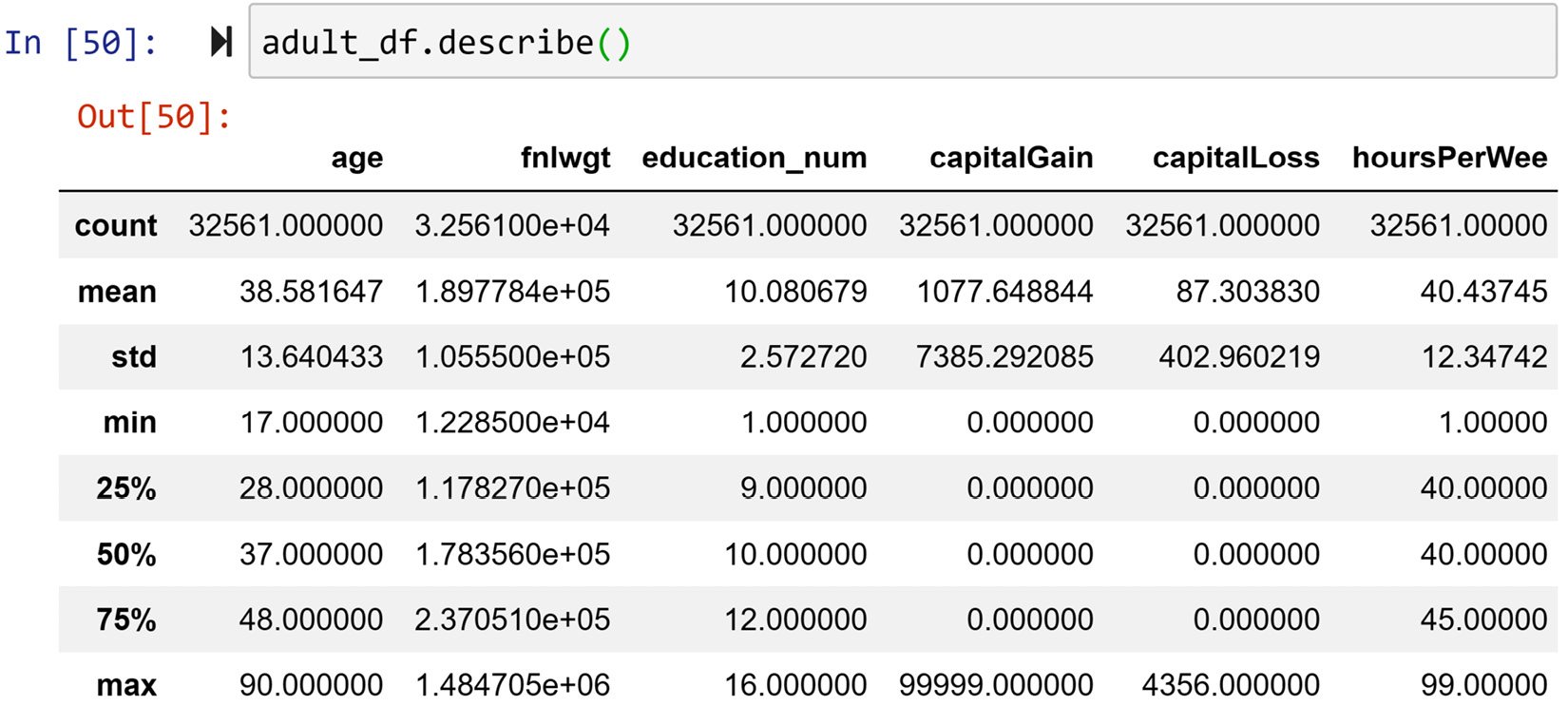
Figure 1.31 – Example of using the .describe() function to get to know a dataset
The metrics that the .describe() function outputs are very valuable summarizing tools, especially if these metrics are meant to be used for algorithmic analytics. However, studying them all at once still overwhelms our human comprehension. To summarize data for human comprehension, there are more effective tools, such as visualizing data using histograms and boxplots.
Histograms and boxplots to visualize numerical columns
Pandas makes drawing these visuals very easy. Each Pandas series has a very useful collection of plot functions. For instance, the following screenshot shows how easy it is to draw the histogram for the age column. To create the boxplot for the age column, all you need to change is the last part of the code: adult_df.age.plot.box(). Give it a try. Also, draw the boxplot and histogram for all of the other numerical attributes and see for yourself how much easy it is to understand each column using visualization.
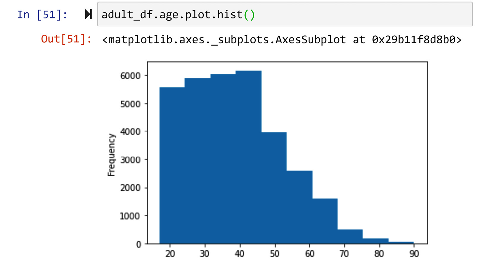
Figure 1.32 – Drawing the histogram of the adult_df.age column
Let's move on to the functions that we will use for categorical attributes. We will start with .unique().
The .unique() function
If the column is categorical, our approach to get to know it would be completely different. First, we need to see what are all the possibilities for the column. The .unique() function does just that. It simply returns all the possible values of the columns. See the following screenshot, which is an example of all the possible values of the relationship column in adult_df:

Figure 1.33 – Example of using the .unique() function to get to know a dataset
Now that we have covered the .unique() function, we will cover the .value_counts() function next.
The .value_counts() function
The next step in getting to know a categorical column is realizing how often each possibility happens. The .value_counts() function does exactly that. The following screenshot shows the outcome of this function on the column's relationship:

Figure 1.34 – Example of using the .value_counts() function to get to know a dataset
The output of the .value_counts() function is also known as the frequency table. There is also the relative frequency table, which shows the ratio of occurrences instead of the number of occurrences for each possibility. To get the relative frequency table, all you need to do is to specify that you want the table to be normalized: .value_counts(normalize=True). Give it a try!
Barcharts for visualizing numerical columns
To draw the bar chart of a categorical attribute, even though you might be tempted to try out something like adult_df.relationship.plot.bar(), it won't work. Give it a try and study the error.
To create the bar chart, you would have to first create the frequency table. As the frequency table is a Pandas series itself, you can then draw the bar chart using that. The following screenshot shows how we can draw the bar chart for the relationship column using the functions .value_counts() and .plot.bar():
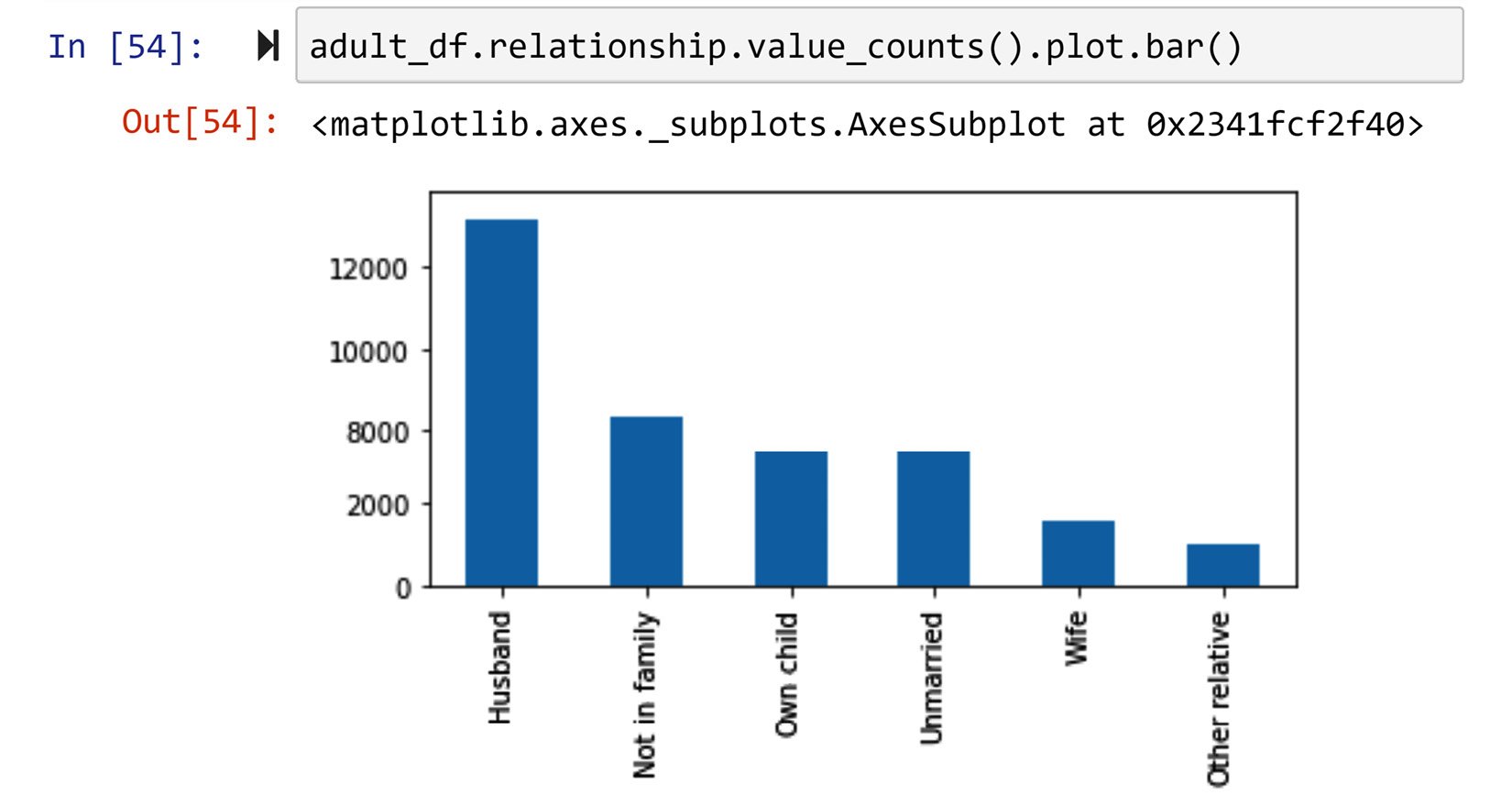
Figure 1.35 – Drawing the bar chart of the adult_df.relationship column
In this part, we learned how we can take advantage of Pandas resources to get to know new datasets. Next, we will learn about a Pandas function that is a game-changer in analyzing and preprocessing data using programming.
Pandas applying a function
There are a lot of instances where we will want to do the same calculations for each row in a dataset. The traditional approach to going about such calculations is to loop through the data and, on every iteration of the loop, perform and save the calculations. Python and Pandas have changed this paradigm by introducing the concept of applying a function. When you apply a function to a DataFrame, you request Pandas to run it for every row.
You can apply a function to a series or a DataFrame. Since applying a function to a series is somewhat easier, we will learn about that first and then we will move on to apply a function to a DataFrame.
Applying a function to a series
Let's say we want to multiply the series adult_df.age by 2. First, you need to write a function that assumes one input as a number, multiply the input by 2, and then output the result. The following screenshot shows this. First, the MutiplyBy2() function is defined, and then, using adult_df.age.apply(MutiplyBy2), is applied to the series.
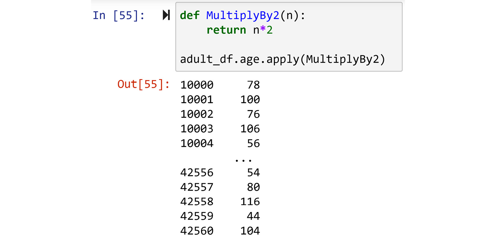
Figure 1.36 – Example of using the .apply() function
Now, let's see an analytic example where the .apply() function can be instrumental.
Applying a function – Analytic example 1
Not only does the series adult_df.fnlwgt not have an intuitive name, but also its values are not easily relatable. As mentioned earlier, the values are meant to be the ratio of the population that each row represents. As the numbers are neither percentages nor the actual number of people that each row represents, these values are neither intuitive nor relatable.
Now that we know how to do a calculation for each value in a series, let's fix this with a simple calculation. How about we divide every value by the sum of all the values in the series?
The following screenshot shows the steps for going about this:
- First,
total_fnlwgt, which is the sum of all the values in thefnlwgtcolumn, is calculated. - Second, the
CalculatePercentagefunction is defined. This function outputs the input values divided bytotal_fnlwgtand multiplied by 100 (to develop a percentage). - Third, the
CalculatePercentagefunction is applied to the seriesadult_df.fnlwgt.
Now, pay attention! Instead of just seeing the results of the calculations, the following code has assigned the result to adult_df.fnlwgt itself, which substitutes the original values with the newly calculated percentages. The following code does not show the output of the code, but give it a try on your Jupyter notebook and study the output on your own:
total_fnlwgt = adult_df.fnlwgt.sum()
def CalculatePercentage(v):
    return v/total_fnlwgt*100
adult_df.fnlwgt = adult_df.fnlwgt.apply(                  CalculatePercentage)
adult_df
Applying a Lambda function
A lambda function is a function that is expressed in one line. So, a lot of the time, applying a lambda function may make coding easier and perhaps help our code become a bit more readable at times. For instance, if you wanted to answer the preceding calculations "on the fly," you could simply apply a lambda function instead of an explicit function. See the following code and compare the simplicity and conciseness of using a lambda function instead of an explicit function:
total_fnlwgt = adult_df.fnlwgt.sum()
adult_df.fnlwgt = adult_df.fnlwgt.apply(lambda v: v/total_fnlwgt*100)
adult_df
It is important to understand that the right choice between a lambda function or an explicit function depends on the situation. Sometimes, having to jam a perhaps complicated function into a line causes coding to become more difficult and renders the code less readable. This will be the case if the function has more than one conditional statement.
Applying a function to a DataFrame
The major difference between applying a function to a DataFrame and a series is when you are defining the function. While, for a series, we had to assume that one value would be input in the function, for a DataFrame, we have to assume that a row series will be input. So, when you are defining a function to apply to a DataFrame, you can engage any column that you need.
For instance, the following code has defined and applied a function that subtracts education_num from age for every column. Pay attention to three aspects:
- First, when defining the
CalcLifeNoEd()function, the input row was assumed to be a row series ofadult_df. In other words, theCalcLifeNoEd()function is tailored just for application toadult_dfor any DataFrame that hasageandeduction_numas columns. - Second, the
.apply()function comes right after the DataFrame itself instead of after any columns. Compare the code for applying a function to a DataFrame to that of a series. Compare the last two code snippets with the following code snippet. - Third, the inclusion of
axis=1is necessary, and what this means is that you want to apply the function to every row and not every column. You could also apply a function to every column. That almost never happens for analytics, but if you ever needed to, you would have to change it toaxis=0.
I have not included the output of this executed code. Give the code a try and study its output:
def CalcLifeNoEd(row):
    return row.age - row.education_num
adult_df.apply(CalcLifeNoEd,axis=1)
This could have easily been done using the lambda function as well. The code that you will need to run is the following. Give it a try:
adult_df.apply(lambda r: r.age-r.education_num,axis=1)
Applying a function – Analytic example 2
Which one is more important in terms of your financial success: education or life experience?
To answer this question, we could use adult_df as a sample dataset and extract some insight from the population of people in 1966. The code in the following screenshot first creates two new columns in the data:
lifeNoEd: The number of years for which you have lived without formal educationcapitalNet: The subtraction ofcapitalLossfromcapitalGain
To answer this question, we can check which one of education_num or lifeNoEd has a higher correlation with capitalNet. Doing this is very easy using Pandas, as each Pandas DataFrame comes with a function, .corr(), which calculates the Pearson correlation coefficient for all the combinations of the numerical attributes in the DataFrame. As we are only interested in the correlations between education_num, lifeNoEd, and capitalNet, the last line of the code has removed other columns before running the .corr() function.
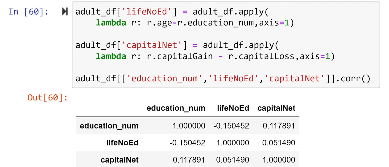
Figure 1.37 – Solution to the preceding example
From the output, you can see that while the correlation between lifeNoEd and capitalNet is 0.051490, the correlation between education_num and capitalNet is higher, at 0.117891. So we have some evidence that education has a more effective role in financial success than just life experience.
Now that you've learned how to effectively apply a function for analytics purposes, we can move on to learn about another very powerful and useful function in Pandas that is invaluable for data analytics and preprocessing.
The Pandas groupby function
This is one of the most useful analytics and preprocessing tools of Pandas. As the name Groupby suggests, it groups your data by something. Normally, you would want to group your data by categorical attributes.
If you are familiar with SQL queries, Pandas groupby is almost identical to SQL groupby. For both SQL queries and Pandas queries, grouping your data by itself will not have any added value or any output, unless it is accompanied by an aggregate function.
For instance, if you want to count the number of rows per marital_status category, you can use the Groupby function. See and try the following code:
adult_df.groupby('marital_status').size()
You can group the DataFrame by more than one column as needed. To do so, you will have to introduce the columns you are grouping the DataFrame by in the form of a list of column names. For instance, the following code groups the data based on both the marital_status and sex columns:
adult_df.groupby(['marital_status','sex']).size()
Pay attention that the two columns are introduced to the function as a list of string values.
The only aggregate function that works without having to specify a column of interest is .size(), as seen above. However, once you specify the column of interest that you want to aggregate the data of, you could use any aggregate function that you can use on a Pandas series or DataFrame. The following table shows a list of all the aggregate functions that you can use:
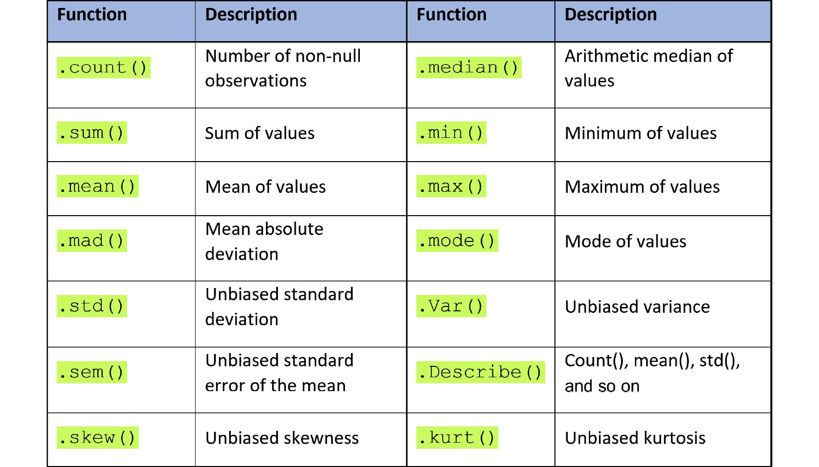
Figure 1.38 – List of Pandas aggregate functions
For instance, the following shows the code to group adult_df by martial_status and sex, and calculates the median of each group:
adult_df.groupby(['marital_status','sex']).age.median()
As you study the code and its output, you can start appreciating the analytic value of the .groupby() function. Next, we will look at an example that will help you appreciate this valuable function even further.
Analytic example using Groupby
Were the race and gender of individuals in 1966 influential in their financial success?
Incidentally, adult_df was collected in 1966, so we can use it to provide some insight into this question. You may take different approaches in going about this. One approach, as depicted in the following screenshot, is to group the data by race and sex and then calculate the mean of capitalNet for the groups and study the differences.
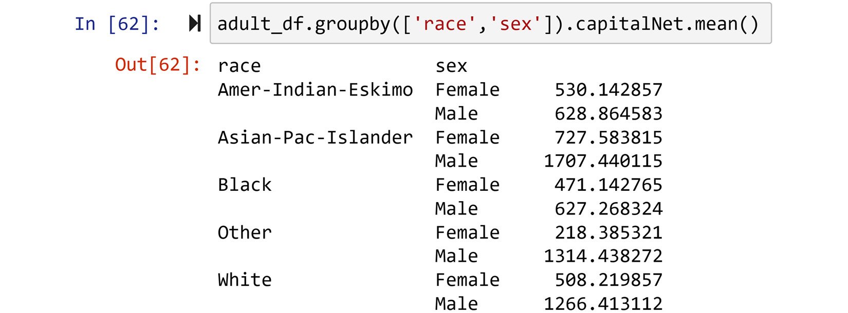
Figure 1.39 – Solution to the preceding example
Another approach would be to group the data based on race, sex, and income and then calculate the mean of fnlwgt. Give this one a try and see whether you come to a different conclusion.
Pandas multi-level indexing
Let's first understand what multi-level indexing is. If you look at the output of grouping a DataFrame by more than one column, the indexing of the output looks different than normal. Although the output is a Pandas series, it looks different. The reason for this dissimilarity is multi-level indexing. The following screenshot shows you the index of the .groupby() output for the previous screenshot. You can see that the index of the series has two levels, specifically, race and sex:
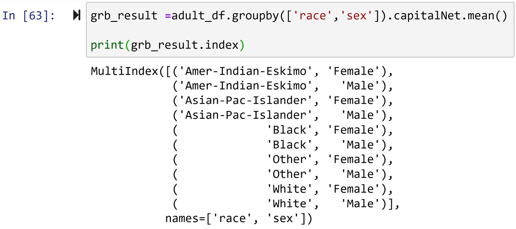
Figure 1.40 – An example of multi-level indexing
Now, let's learn a few useful and relevant functions that can help us with data analytics and preprocessing. These functions are .stack() and .unstack().
The .unstack() function
This function pushes the outer level of the multi-level index to the columns. If the multi-level index only has two levels, after running .unstack(), it will become single-level. Likewise, if the .unstack() function is run for a series with a multi-level index, the output will be a DataFrame whose columns are the outer level index that was pushed. For instance, the following screenshot demonstrates the change in appearance and structure of the output when the .unstack() function is executed:
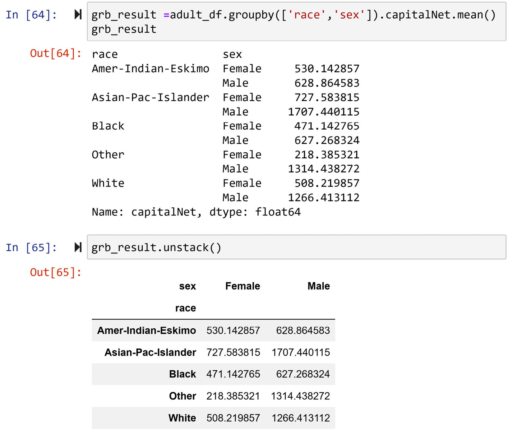
Figure 1.41 – Example of the .unstack() function
If there are more than two levels, executing .unstack() more than once will, one by one, push the outer level of the index to the columns. For instance, you can see in the following screenshot that the code in the first chunk results in grb_result, which is a series with a three-level index. The second chunk of code executes .unstack() once and the outer level of the index in grb_result, which is income, is pushed to the columns. The third chunk of code, however, executes .unstack() twice, and the second outer level of the index in grb_result, which is sex, joins income in the columns.
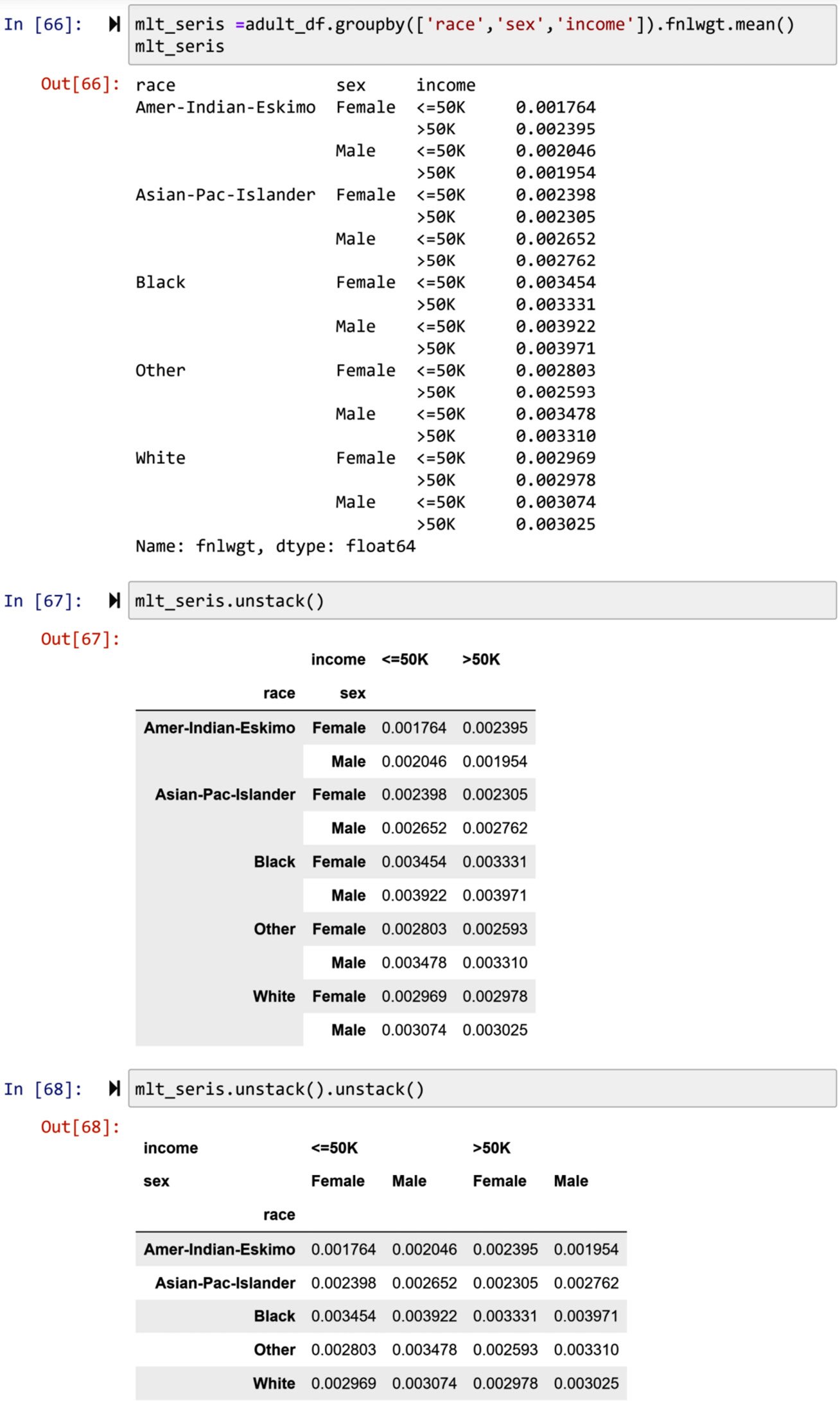
Figure 1.42 – Another example of the .unstack() function with two levels of indexing
As an index can be multi-level in Pandas, columns can also have multiple levels. For instance, in the first chunk of the following screenshot, you can see that the output DataFrame has two levels. The second chunk of code outputs the columns of the DataFrame. You can see that the columns have the two levels that were pushed from the index using .unstack():
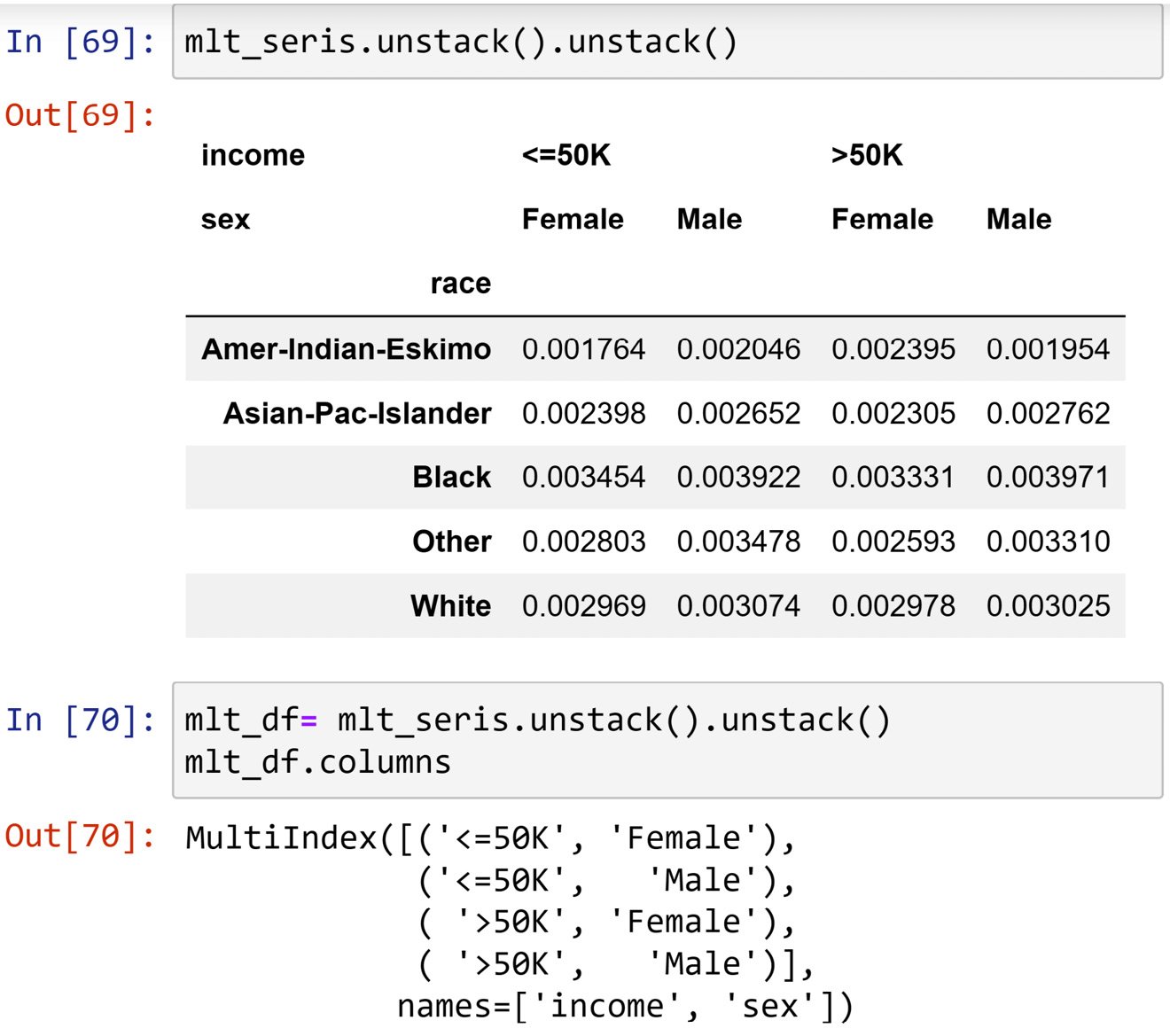
Figure 1.43 – An example of multi-level columns
The .stack() function
The opposite of .unstack() is .stack(), where the outer level of the columns is pushed to be added as the outer level of the index. For example, in the following screenshot, you can see that mlt_df, which we saw has two-level columns, has undergone .stack() twice. The first .stack() function pushed the income level to the index, and the second .stack() function pushed the sex level to the index. This made the data be presented as a series as there is only one column of data.
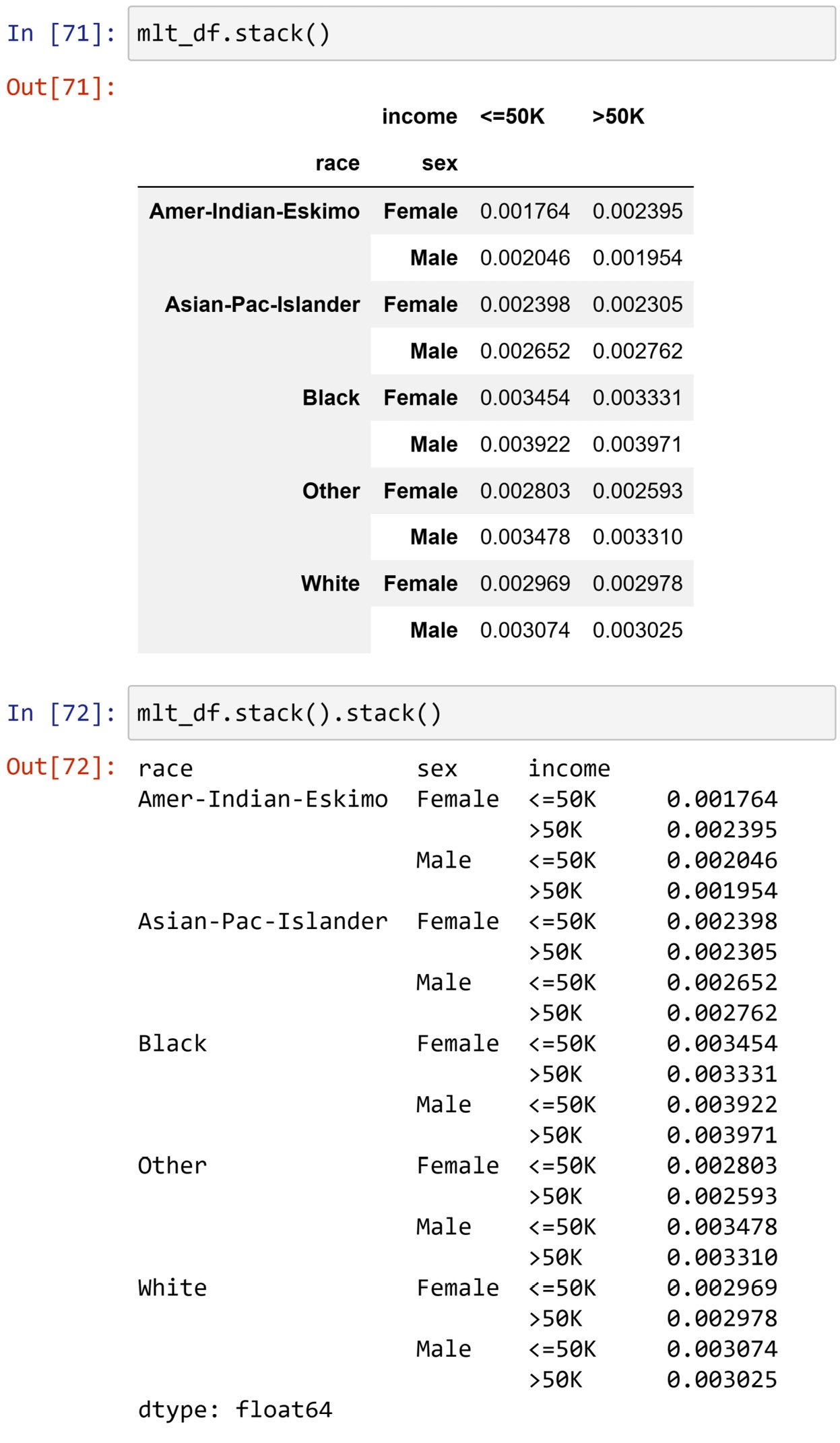
Figure 1.44 – Example of the .stack() function
Multi-level access
The value access in series or DataFrames with multi-level indexes, or DataFrames with multi-level columns, is slightly different. Exercise 2 at the end of this chapter is designed to help you learn that.
In this subsection, we gathered sizable exposure to multi-level indexing and columns. Now we are moving on to another set of functions that are somewhat similar to the .stack() and .unstack() functions, but different at the same time. These functions are .pivot() and .melt().
Pandas pivot and melt functions
In a nutshell, .pivot() and .melt() help you to switch between two forms of two-dimensional data structures: wide form and long form. The following figure depicts the difference between the two forms. The wide form is what you are typically used to if you are a spreadsheet user. The wide form uses many columns to introduce new dimensions in the dataset. The long form, however, uses a different logic of data structure and uses one index column to include all the relevant dimensions. The .melt() function, as you may picture it in your mind based on the meaning of the word melt, can easily reshape a dataset from the wide form to the long form. The .pivot() function can do the opposite.
To practice and learn these two functions, we will read wide.csv using Pandas into wide_df, and read long.csv using Pandas into long_df.
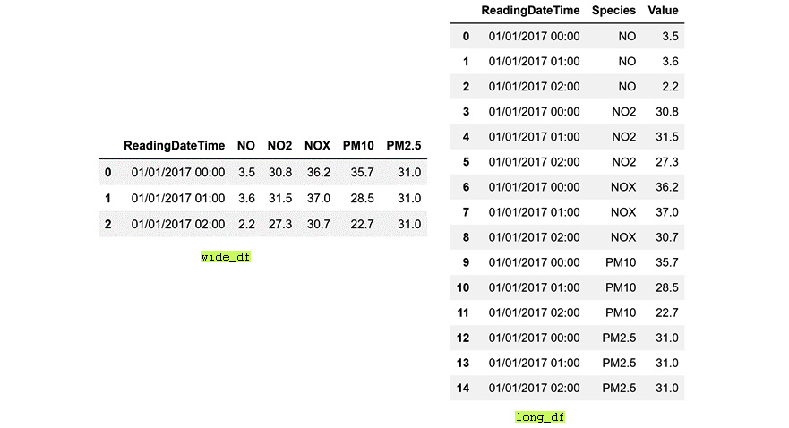
Figure 1.45 – Comparison of the long and wide forms
To switch between the long and the wide format, all you need to do is to provide the right input to these functions. The following screenshot shows the application of .melt() on wide_df, reshaping it into a long format. In the second chunk of code, you can see that .melt() requires four inputs:
id_vars: This input takes the identifying columns.value_vars: This input takes the columns that hold the values.var_name: This input takes the name you would like to give to the identifying column that will be added to the long format.value_name: This input takes the name you would like to give to the new value column that will be added to the long format.
The following screenshot shows an example of using the .melt() function to switch the data from wide format to long format:
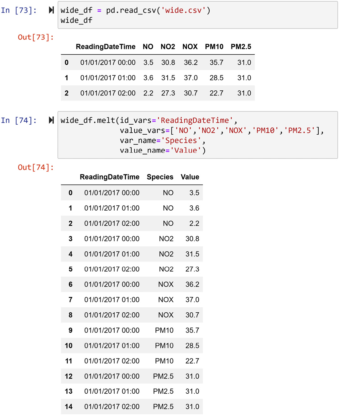
Figure 1.46 – Example of using the .melt() function to switch the data from wide format to long format
The .pivot() function reshapes a DataFrame from the long form to the wide form. For instance, the following screenshot shows the application of the function on long_df. Unlike, .melt(), which requires four inputs, .pivot() needs three:
index: This input takes what will be the index of the wide form.columns: This input takes the columns of the long form that will be expanded to create the columns for the wide form.values: This input takes the column in which the long form keeps the values.
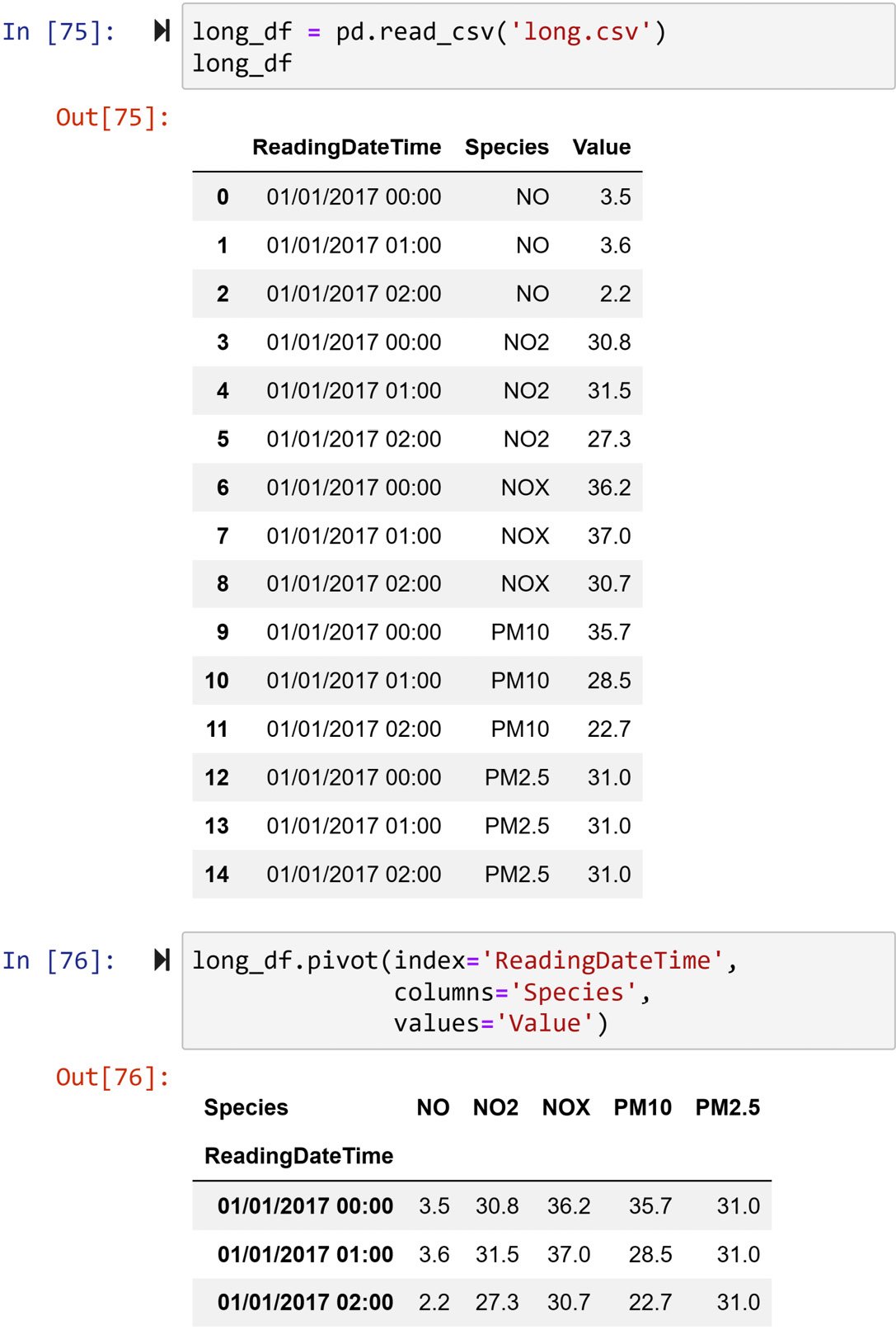
Figure 1.47 – Example of using the .pivot() function to switch the data from the long format to the wide format


