In this recipe, we will test out some well-known models (ARIMA, SARIMA) and signal decomposition by forecasting using Facebook's Prophet library on the time series data, in order to check their performance at forecasting our time series of CO2 values.
Getting ready
In order to prepare for this recipe, we'll install libraries and download a dataset.
We'll use the statsmodels package and prophet:
pip install statsmodels fbprophet
We will analyze the CO2 concentration data in this recipe. You can see the data loading in the notebook on GitHub accompanying this recipe, or in the scikit-learn Gaussian process regression (GPR) example regarding Mauna Loa CO2 data: https://scikit-learn.org/stable/auto_examples/gaussian_process/plot_gpr_co2.html#sphx-glr-auto-examples-gaussian-process-plot-gpr-co2-py
This dataset is one of the earliest recordings available on atmospheric recordings of CO2. As it will be later observed, this data follows a sinusoidal pattern, with the CO2 concentration rising in winter and falling in the summer owing to the decreasing quantity of plants and vegetation in the winter season:
X,y = load_mauna_loa_atmospheric_co2()The dataset contains the average CO2 concentration measured at Mauna Loa Observatory in Hawaii from 1958 to 2001. We will model the CO2 concentration with respect to that.
How to do it...
Now we'll get to forecasting our time series of CO2 data. We'll first explore the dataset, and then we'll apply the ARIMA and SARIMA techniques.
- Let's have a look at the time series:
df_CO2 = pd.DataFrame(data = X, columns = ['Year'])
df_CO2['CO2 in ppm'] = y
lm = sns.lmplot(x='Year', y='CO2 in ppm', data=df_CO2, height=4, aspect=4)
fig = lm.fig
fig.suptitle('CO2 conc. mauna_loa 1958-2001', fontsize=12)
Here's the graph:

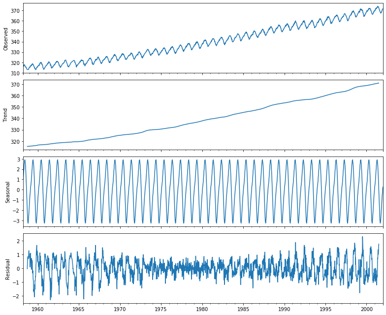
The script here shows the time series seasonal decomposition of the CO2 data, showing a clear seasonal variation in the CO2 concentration, which can be traced back to the biology:
import statsmodels.api as stmd
d = stm.datasets.co2.load_pandas()
co2 = d.data
co2.head()
y = co2['co2']
y = y.fillna(
    y.interpolate()
)  # Fill missing values by interpolation
Now that we have preprocessed data for decomposition, let's go ahead with it:
from pylab import rcParams
rcParams['figure.figsize'] = 11, 9
result = stm.tsa.seasonal_decompose(y, model='additive')
pd.plotting.register_matplotlib_converters()
result.plot()
plt.show()
Here, we see the decomposition: the observed time series, its trend, seasonal components, and what remains unexplained, the residual element:
Now, let's analyze the time series.
Analyzing time series using ARIMA and SARIMA
We will fit ARIMA and SARIMA models to the dataset.
We'll define our two models and apply them to each point in the test dataset. Here, we iteratively fit the model on all the points and predict the next point, as a one-step-ahead.
- First, we split the data:
# taking a 90/10 split between training and testing:
future = int(len(y) * 0.9)
print('number of train samples: %d test samples %d' (future, len(y)-future)
)
train, test = y[:future], y[future:]
This leaves us with 468 samples for training and 53 for testing.
- Next, we define the models:
from statsmodels.tsa.arima_model import ARIMA
from statsmodels.tsa.statespace.sarimax import SARIMAX

def get_arima_model(history, order=(5, 1, 0)):
    return ARIMA(history, order=order)

def get_sarima_model(
    history,
    order=(5, 1, 1),
    seasonal_order=(0, 1, 1, 4)
    ):
    return SARIMAX(
        history,
        order=order,
        enforce_stationarity=True,
        enforce_invertibility=False,
        seasonal_order=seasonal_order
    )
- Then we train the models:
from sklearn.metrics import mean_squared_error

def apply_model(train, test, model_fun=get_arima_model):
  '''we just roll with the model and apply it to successive
  time steps
  '''
  history = list(train)
  predictions = []
  for t in test:
    model = model_fun(history).fit(disp=0)
    output = model.forecast()
    predictions.append(output[0])
    history.append(t)
  error = mean_squared_error(test, predictions)
  print('Test MSE: %.3f' % error)
  #print(model.summary().tables[1])
  return predictions, error

predictions_arima, error_arima = apply_model(train, test)
predictions_sarima, error_sarima = apply_model(
    train, test, get_sarima_model
)
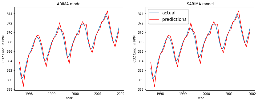
We get an MSE in the test of 0.554 and 0.405 for ARIMA and SARIMA models, respectively. Let's see how the models fit graphically:
We could do a parameter exploration using the Akaike information criterion (AIC), which expresses the quality of the model relative to the number of parameters in the model. The model object returned by the fit function in statsmodels includes the AIC, so we could do a grid search over a range of parameters, and then select the model that minimizes the AIC.
How it works...
Time series data is a collection of observations x(t), where each data point is recorded at time t. In most cases, time is a discrete variable, that is,  . We are looking at forecasting, which is the task of predicting future values based on the previous observations in the time series.
In order to explain the models that we've used, ARIMA and SARIMA, we'll have to go step by step, and explain each in turn:
- Autoregression (AR)
- Moving Average (MA)
- Autoregressive Moving Average (ARMA)
- Autoregressive Integrated Moving Average (ARIMA) and
- Seasonal Autoregressive Integrated Moving Average (SARIMA)
ARIMA and SARIMA are based on the ARMA model, which is an autoregressive moving average model. Let's briefly go through some of the basics.
ARMA is a linear model, defined in two parts. First, the autoregressive linear model:

Here,  are parameters and
  is a constant,
  is white noise, and
  is the order of the model (or the window size of the linear model). The second part of ARMA is the moving average, and this is again a linear regression, but of non-observable, lagged error terms, defined as follows:

Here,  is the order of the moving average,
  are the parameters, and
  the expectation or the mean of the time series
  . The ARMA(p, q) model is then the composite of both of these models, AR(p) and MA(q):

The fitting procedure is a bit involved, particularly because of the MA part. You can read up on the Box-Jenkins method on Wikipedia if you are interested: https://en.wikipedia.org/wiki/Box%E2%80%93Jenkins_method
There are a few limitations to note, however. The time series has to be the following:
- Stationary: Basically, mean and covariance across observations have to be constant over time.
- Nonperiodic: Although bigger values for p and q could be used to model seasonality, it is not part of the model.
- Linear: Each value for
 can be modeled as a linear combination of previous values and error terms.
There are different extensions of ARMA to address the first two limitations, and that's where ARIMA and SARIMA come in.
ARIMA (p, d, q) stands for autoregressive integrated moving average. It comes with three parameters:
- p: The number of autoregressive terms (autoregression)
- d: The number of non-seasonal differences needed for stationarity (integration)
- q: The number of lagged forecast errors (moving average)
The integration refers to differencing. In order to stabilize the mean, we can take the difference between consecutive observations. This can also remove a trend or eliminate seasonality. It can be written as follows:

This can be repeated several times, and this is what the parameter d describes that ARIMA comes with. Please note that ARIMA can handle drifts and non-stationary time series. However, it is still unable to handle seasonality.
SARIMA stands for seasonal ARIMA, and is an extension of ARIMA in that it also takes into account the seasonality of the data.
SARIMA(p, d, q)(P, D, Q)m contains the non-seasonal parameters of ARIMA and additional seasonal parameters. Uppercase letters P, D, and Q annotate the seasonal moving average and autoregressive components, where m is the number of periods in each season. Often this is the number of periods in a year; for example m=4 would stand for a quarterly seasonal effect, meaning that D stands for seasonal differencing between observations Xt and Xt-m, and P and Q stand for linear models with backshifts of m.
In Python, the statsmodels library provides a method to perform the decomposition of the signal based on the seasonality of the data.
There's more...
Prophet is a library provided by Facebook for forecasting time series data. It works on an additive model and fits non-linear models. The library works best when the data has strong seasonal effects and has enough historic trends available.
Let's see how we can use it:
from fbprophet import Prophet

train_df = df_CO2_fb['1958':'1997']
test_df = df_CO2_fb['1998':'2001']
train_df = train_df.reset_index()
test_df = test_df.reset_index()Co2_model= Prophet(interval_width=0.95)

Co2_model.fit(train_df)
train_forecast = Co2_model.predict(train_df)
test_forecast = Co2_model.predict(test_df)
fut = Co2_model.make_future_DataFrame(periods=12, freq='M')
forecast_df = Co2_model.predict(fut)
Co2_model.plot(forecast_df)
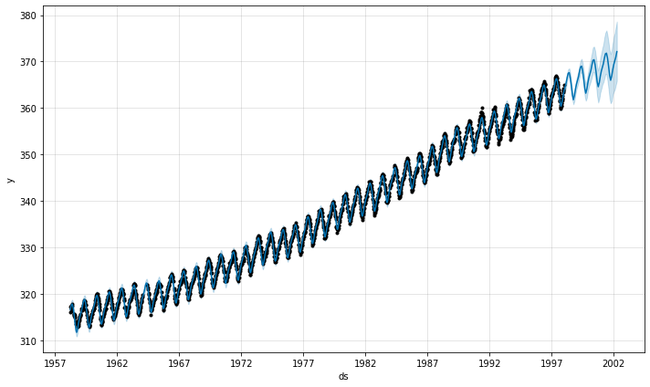
Here are our model forecasts:
We get a similar decomposition as before with the ARIMA/SARIMA models, namely, the trend and the seasonal components:
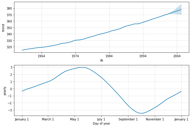
The yearly variation nicely shows the rise and fall of the CO2 concentration according to the seasons. The trend clearly goes up over time, which could be worrisome if you think about global warming.
See also
We've used the following libraries in this recipe:
- Statsmodels: http://statsmodels.sourceforge.net/stable/
- Prophet: https://facebook.github.io/prophet/
There are many more interesting libraries relating to time series, including the following:
- Time series modeling using state space models in statsmodels:
https://www.statsmodels.org/dev/statespace.html - GluonTS: Probabilistic Time Series Models in MXNet (Python): https://gluon-ts.mxnet.io/
- SkTime: A unified interface for time series modeling: https://github.com/alan-turing-institute/sktime


