Characteristics of a machine learning model
In this section, we're mainly going to consider supervised models, even though the concepts we'll discuss are valid in general. We'll try to determine how it's possible to measure the theoretical potential accuracy of a model, and a model's ability to generalize correctly over every possible sample drawn from pdata.
The majority of these concepts were developed long before the deep learning age, but continue to have an enormous influence on research projects.
The idea of capacity, for example, is an open-ended question that neuroscientists keep on asking themselves about the human brain. Modern deep learning models with dozens of layers and millions of parameters have reopened this theoretical question from a mathematical viewpoint. Together with this, other elements, such as the limits for the variance of an estimator, have again attracted the limelight because the algorithms are becoming more and more powerful, and performances that once were considered far from feasible are now a reality.
Being able to train a model, so as to exploit its full capacity, maximize its generalization ability, and increase its accuracy to overcome even human performances, is what a modern data scientist or deep learning engineer ought to expect from their work.
Learnability
Before starting the discussion of the features of a model, it's helpful to introduce some fundamental elements related to the concept of learnability, work not too dissimilar from the mathematical definition of generic computable functions. The first formal work on this was published by Valiant (in Valiant L., A theory of the learnable, Communications of the ACM, 27, 1984) and is mostly an introduction of the concept of Probably Approximately Correct (PAC) learning. We won't discuss the very technical mathematical details of PAC learning in this book, but it's useful to understand the possibility of finding a suitable way to describe a learning process, without referring to specific models.
For simplicity, let's assume we have a selector algorithm that can search a hypothesis hi in a set H. This element can be interpreted in many ways according to the context. For example, the set of hypotheses might correspond to the set of reasonable parameters of a model, or, in another scenario, to a finite set of algorithms tuned to solve specific problems. As the definition is general, we don't have to worry about its structure.
On the other side of this landscape, there is the set of concepts C that we want to learn. A concept  is an instance of a problem belonging to a defined class. Again, the structure can vary, but for simplicity the reader can assume that a concept is associated with a classical training set containing a finite number of data points.
For our purposes, it's necessary to define the structure of an error measure (we're going to do that later, when talking about cost and loss functions). If you're not familiar with the concept, it's possible to consider the normalized average number of misclassified data points.
If the sample size is N, an error equal to 0 implies that there are no misclassifications, while an error equal to 1 means that all the samples have been misclassified. Just as for AUC diagrams, in a binary classifier we consider the threshold of 0.5 as lower bound, because it corresponds to a random choice of the label.
An informal definition states that a problem is PAC learnable if, given a desired maximum error  and probability
  , it's possible to set a minimum sample size N for every concept
  , so that a selector algorithm can find a hypothesis
  such that the probability that the error is upper bounded by
  is greater than
  .
.
As the problem is generally stochastic, the result must be expressed using probabilities. That means we can summarize the previous definition, saying that for a PAC learnable problem,  . We also need to add that we expect the sample to have polynomial growth as a function of
  and
and  . This condition can be relaxed with respect to the original one, but it's enough to understand that a problem that requires an infinite sample size to achieve an error greater than 0 is not PAC learnable.
This characterization justifies the use of the word approximately in the definition, which could lead to misunderstandings if not fully mathematically defined. In our context, in fact, we cope with deterministic problems very rarely, and they generally don't require a machine learning algorithm. It's more helpful to know that the probability of obtaining a small error is always larger than a predefined threshold. Even if the theory is much more complex and rigorous, we can avoid all the theoretical details (which are available in Valiant's paper mentioned before) and limit our analysis to this concrete meaning of the concept.
Given a problem, we can generally find a model that can learn the associated concept and keep the accuracy above a minimum acceptable value. That's equivalent to saying that the concept is PAC learnable, a condition that we haven't proved, but that can reasonably be assumed to be true in most real-life contexts. Therefore, taking the PAC learnability for granted, we know that we can reach the desired accuracy for a specific scenario.
However, the price to pay for that isn't so easy to evaluate. For sure, when the requirements become stronger and stronger, we also need a larger training set and a more powerful model, but is this enough to achieve an optimal result? Moreover, is it possible to quantify how optimal the result is using a single measure? In the next sections, we'll introduce the elements that must be evaluated when defining, or evaluating, every machine learning model.
Capacity of a model
If we consider a supervised model as a set of parameterized functions, we can define the representational capacity as the intrinsic ability of a certain generic function to map a relatively large number of data distributions. To understand this concept, let's consider a function f(x) that admits infinite derivatives, and rewrite it as a Taylor expansion around a starting point x0:

We can decide to take only the first n terms, so to have an n-degree polynomial function around the starting point x0 = 0:

Consider a simple bi-dimensional scenario with six functions, starting from a linear one. We can observe the different behaviors with a small set of data points:
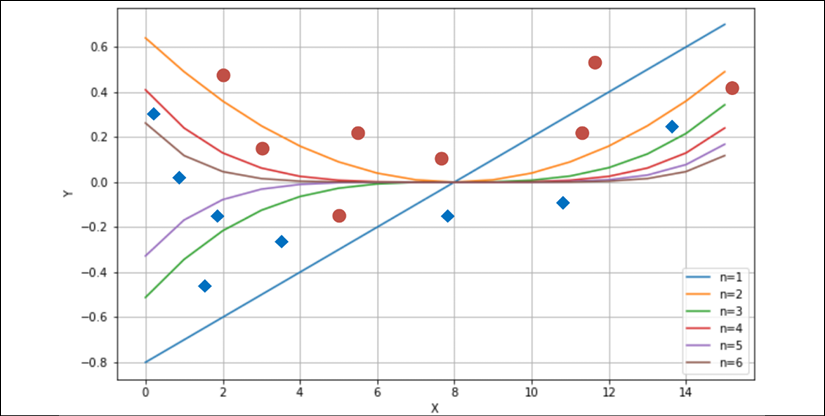
Different behavior produced by six polynomial separating curves
The ability to rapidly change the curvature is proportional to the degree. If we choose a linear classifier, we can only modify its slope—the example is always in a bi-dimensional space—and the intercept.
Instead, if we pick a higher-degree function, we have more possibilities to bend the curvature when it's necessary. If we consider n=1 and n=2 in the plot (on the top-right, they are the first and the second functions), with n=2, we can include the dot corresponding to x=11, but this choice has a negative impact on the dot at x=5.
Only a parameterized non-linear function can solve this problem efficiently. That's because this simple problem requires a representational capacity higher than the one provided by linear classifiers. Another classical example is the XOR function. For a long time, several researchers opposed perceptrons (linear neural networks) because they couldn't classify a dataset generated by the XOR function.
Fortunately, the introduction of Multilayer Perceptrons (MLP), with non-linear functions, allowed us to overcome this problem, and many other problems whose complexity is beyond the possibilities of any classic machine learning model. For a better understanding of this concept, it's helpful to introduce a formalism that allows us to understand how different model families treat the same kind of problem, achieving better or worse accuracies.
Vapnik-Chervonenkis capacity
A common mathematical formalization of the capacity of a classifier is provided by the Vapnik-Chervonenkis theory. To introduce the definition, it's first necessary to define the concept of shattering. If we have a class of sets C and a set M, we say that C shatters M if:

In other words, given any subset of M, it can be obtained as the intersection of a particular instance of C (cj) and M itself. Now, if we consider a model as a parameterized function:

Considering the variability of  , C can be considered as a set of functions with the same structure, but different parameters:

We want to determine the capacity of this model family in relation to a finite dataset X:

According to the Vapnik-Chervonenkis theory, we can say that the model family C shatters X if there are no classification errors for every possible label assignment. Therefore, we can define the Vapnik-Chervonenkis-capacity or VC-capacity—sometimes called VC-dimension—as the maximum cardinality of a subset of X, so that any  can shatter it (that is, the maximum number of points that
  can shatter).
For example, if we consider a linear classifier in a bi-dimensional space, the VC-capacity is equal to 3, because it's always possible to label three samples so that  shatters them. However, it's impossible to do it in all situations where N > 3. The XOR problem is an example that needs a VC-capacity higher than three. Let's explore the following plot:
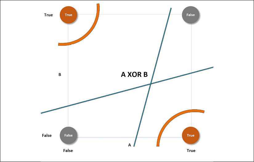
XOR problem with different separating curves
This particular label choice makes the set non-linearly separable. The only way to overcome this problem is to use higher-order functions, or non-linear ones. The curve lines—belonging to a classifier whose VC-capacity is greater than 3—can separate both the upper-left and the lower-right regions from the remaining space, but no straight line can do the same, although it can always separate one point from the other three.
This definition of capacity is quite rigorous (the reader who's interested in the all theoretical aspects can read Mohri M., Rostamizadeh A., Talwalkar A., Foundations of Machine Learning, Second edition, The MIT Press, 2018), but it can help understand the relation between the complexity of a dataset and a suitable model family. According to the principle of Occam's razor, the simplest model that obtains an optimal accuracy (that is, the optimal set of measures that quantifies the performances of an algorithm) must be selected, and in this book, we are going to repeat this principle many times. However, the reason for this advice, which is strictly connected to the informal definition of PAC learning, will become obvious after having introduced the concepts of bias and variance of an estimator.
Bias of an estimator
Let's now consider a parameterized model with a single vectoral parameter. This isn't a limitation, just a didactic choice:

The goal of a learning process is to estimate the parameter  so as, for example, to maximize the accuracy of its classifications. We define the bias of an estimator in relation to a parameter
  :
:

In other words, the bias of  is the difference between the expected value of the estimation and the real parameter value. Remember that the estimation is a function of X, and cannot be considered a constant in the sum.
An estimator is said to be unbiased if:

Moreover, the estimator is defined as consistent if the sequence of estimations  of
of  converges in probability to the real value when
  (that is, it is asymptotically unbiased):

It's obvious that this definition is weaker than the previous one, because in this case, we're only certain of achieving unbiasedness if the sample size becomes infinitely large. However, in practice, many asymptotically unbiased estimators can be considered unbiased when k > Nk. In other words, with samples containing at least Nk points, the results have a negligible error, and the estimation can be considered correct. From the theory, we know that some model families are unbiased (for example, linear regressions optimized using the ordinary least square), but confirming a model is unbiased is extremely different to test when the model is very complex.
For example, we can suppose that a deep neural network is prone to be unbiased, but as we are going to discuss throughout the book, the sample size is a fundamental parameter in achieving good results. Given a dataset X whose samples are drawn from pdata, the accuracy of an estimator is inversely proportional to its bias. Low-bias (or unbiased) estimators are able to map the dataset X with high-precision levels, while high-bias estimators are very likely to have too low a capacity for the problem to solve, and therefore their ability to detect the whole dynamic is poor.
This also implies that, in many cases, if k << Nk, the sample doesn't contain enough of the representative elements that are necessary to rebuild the data generating process, and the estimation of the parameters risks becoming clearly biased. Remember that the training set X is drawn from pdata and contains a limited number of points. Hence, given k different sets X1, X2, ..., Xk obtained from the same data generating process, we are interested in understanding whether the initial estimation is still valid.
If X is truly representative of pdata and the estimator is unbiased, we should expect to always obtain the same mean, with a reasonable tolerance. This condition assures that, at least on average, the estimator yields results distributed around the true values. Let's now consider the extremes of this process: underfitting and overfitting a model.
Underfitting
A model with a large bias is likely to underfit the training set X (that is, it's not able to learn the whole structure of X). Let's consider the simple bidimensional scenario shown in the following figure:
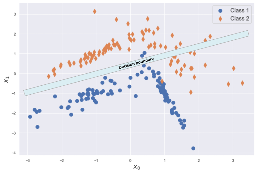
Underfitted classifier: The curve cannot separate correctly the two classes
Even if the problem is very hard, we could try to adopt a linear model and, at the end of the training process, the slope and the intercept of the separating line are about 1 and -1, as shown in the plot. However, if we measure the accuracy, we discover that it's not as large as expected—indeed, it's about 0.65—because there are too many class 2 samples in the region assigned to class 1.
Moreover, the sample size of 200 points is quite small and, therefore, X cannot be a true representative of the underlying data generating process. Considering the density for class 2 observed in the area x0 < 0 and 1 < x1 < 2, it's reasonable to suppose that larger sample size could lead to a worse accuracy due to the increased number of misclassified class 2 points. Independent of the number of iterations, this model will never be able to learn a good association between X and Y.
This condition is called underfitting, and the major indicator of underfitting is very low training accuracy. Unfortunately, even if some data preprocessing steps can improve the accuracy, when a model is underfitted, the only valid solution is to adopt a higher-capacity model. In fact, when the estimation of the parameters is biased, its expected value is always different from the true value. That difference leads to a systematic prediction error that cannot be corrected.
Considering the previous example, a linear model (for example, a logistic regression) can only modify the slope and the intercept of the separating line. The reader can easily see that the number of degrees of freedom are too small to achieve, for example, an accuracy greater than 0.95. Instead, using a polynomial classifier (for example, a parabolic one), the problem can be easily solved. The introduction of another parameter. the coefficient of the square term, allows defining a curve separating line that surely leads to a better fit. Of course, the price to pay is double:
- A model with larger capacity needs a higher computational effort. This is often a secondary problem.
- The extra capacity could reduce the generalization ability, if X is not fully representative of pdata (we are going to discuss this problem in the next section).
In a machine learning task, our goal is to achieve the maximum accuracy, starting from the training set and then moving on to the validation set. More formally, we can say that we want to improve our models so to get as close as possible to Bayes error, which is the theoretical minimal generalization error achievable by an estimator. It can also be expressed as Bayes accuracy, which is the maximum achievable generalization accuracy.
In the following diagram, we can see a representation of this process:
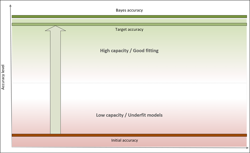
Accuracy level diagram
Bayes accuracy is often a purely theoretical limit and, for many tasks, it's almost impossible to achieve, even using biological systems. However, advancements in the field of deep learning allow creating models that have a target accuracy slightly below the Bayes one. In general, there's no closed form for determining the Bayes accuracy, therefore human abilities are considered as a benchmark.
In the previous classification example, a human being is immediately able to distinguish among different dot classes, but the problem can be very hard for a limited-capacity classifier. Some of the models we're going to discuss can solve this problem with a very high target accuracy, but at this point, we need to introduce the concept of variance of an estimator in order to understand the effects of excessive capacity.
Variance of an estimator
At the beginning of this chapter, we defined the data generating process pdata, and we've assumed that our dataset X has been drawn from this distribution. However, we don't want to learn existing relationships limited to X; we expect our model to be able to generalize correctly to any other subset drawn from pdata. A good measure of this ability is provided by the variance of the estimator:

The variance can be also defined as the square of the standard error, analogously to the standard deviation. A large variance implies dramatic changes in accuracy when new subsets are selected. In fact, even if the model is unbiased, and the estimated values of the parameters are spread around the true mean, they can show high variability.
For example, suppose that an estimated parameter  and the true mean is actually 0. We know that the probability
  ; hence, if a wrong estimation that
  can lead to a significant error, there's a very high risk of misclassification with the majority of validation samples. This effect is related to the fact that the model has probably reached a very high training accuracy through over-learning a limited set of relationships, and it has almost completely lost its ability to generalize (that is, the average validation accuracy decays when never-seen samples are tested).
However, if it's possible to obtain unbiased estimators, it's almost impossible to reduce the variance under a well-defined threshold (see the later section related to the Cramér-Rao bound). Before discussing the implications of the variance, we need to introduce the opposite extreme situation to underfitting: overfitting a model.
Overfitting
If underfitting was the consequence of low capacity and large bias, overfitting is a phenomenon strictly related to large variance. In general, we can observe a very high training accuracy (even close to the Bayes level), but not a poor validation accuracy.
This means that the capacity of the model is high enough or even excessive for the task (the higher the capacity, the higher the probability of large variances), and that the training set isn't a good representation of pdata. To understand the problem, consider the following classification scenarios:
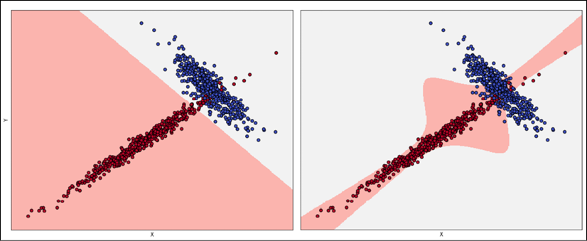
Acceptable fitting (left), overfitted classifier (right)
The left plot has been obtained using logistic regression, while the right plot was obtained with an SVM algorithm with a sixth-degree polynomial kernel. If we consider the second model, the decision boundaries seem much more precise, with some samples just over them. Considering the shapes of the two subsets, it would be possible to say that a non-linear SVM can better capture the dynamics; however, if we sample another dataset from pdata and the diagonal tail becomes wider, logistic regression continues to classify the points correctly, while the SVM accuracy decreases dramatically.
The second model is very likely to be overfitted, and some corrections are necessary. When the validation accuracy is much lower than the training one, a good strategy is to increase the number of training samples, to consider the real pdata. In fact, it can happen that a training set is built starting from a hypothetical distribution that doesn't reflect the real one, or the number of samples used for the validation is too high, reducing the amount of information carried by the remaining samples.
Cross-validation is a good way to assess the quality of datasets, but it can always happen that we misclassify completely new subsets (for example, generated when the application is deployed in a production environment), even if they were supposed to belong to pdata. If it's not possible to enlarge the training set, data augmentation could be a valid solution, because it allows creating artificial samples (for images, it's possible to mirror, rotate, or blur them) starting from the information stored in the known ones.
Other strategies to prevent overfitting are based on a technique called regularization, which we're going to discuss in the next chapter. For now, we can say that the effect of regularization is similar to a partial linearization, which implies a capacity reduction with a consequent variance decrease and a tolerable bias increase.
The Cramér-Rao bound
If it's theoretically possible to create an unbiased model, even asymptotically, this is not true for the variance. To understand this concept, it's necessary to introduce an important definition: the Fisher information. If we have a parameterized model and a data-generating process pdata, we can define a likelihood function by considering the following parameters:

This function allows us to measure how well the model describes the original data generating process. The shape of the likelihood can vary substantially, from well-defined, peaked curves, to almost flat surfaces. Let's consider the following graph, showing two examples based on a single parameter. The x-axis represents the value of a generic parameter, while the y-axis is the log-likelihood:
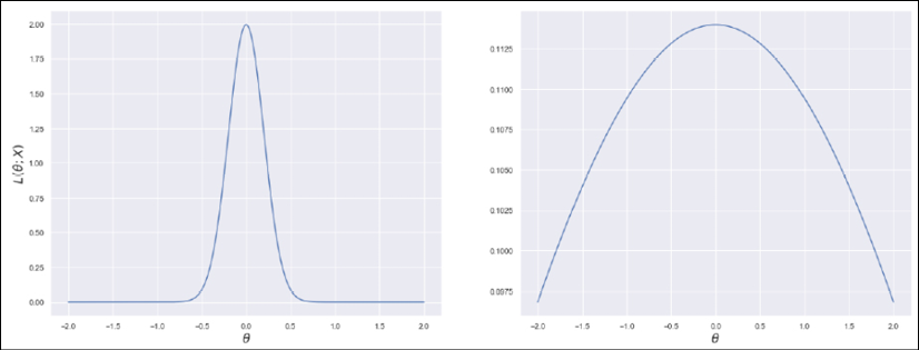
Very peaked likelihood (left), flatter likelihood (right)
We can immediately understand that, in the first case, the maximum likelihood (which represents the value for which the model has the highest probability to generate the training dataset – the concept will be discussed in a dedicated section) can be easily reached using classic optimization methods, because the surface is very peaked. In the second case, instead, the gradient magnitude is smaller, and it's rather easy to stop before reaching the actual maximum because of numerical imprecisions or tolerances. In worst cases, the surface can be almost flat in very large regions, with a corresponding gradient close to zero.
Of course, we'd like it if we could always work with very sharp and peaked likelihood functions, because they carry more information about their maximum. More formally, the Fisher information quantifies this value. For a single parameter, it is defined as follows:

The Fisher information is an unbounded, non-negative number, that is proportional to the amount of information carried by the log-likelihood; the use of logarithm has no impact on the gradient ascent, but it simplifies complex expressions by turning products into sums.
This value can be interpreted as the speed of the gradient when the function is reaching the maximum; therefore, higher values imply better approximations, while a hypothetical value of zero means that the probability to determine the right parameter estimation is also null.
When working with a set of K parameters, the Fisher information becomes a positive semidefinite matrix:

This matrix is symmetrical, and also has another important property: when a value is zero, it means that the corresponding parameters are orthogonal for the purpose of the maximum likelihood estimation, and they can be considered separately. In many real cases, if a value is close to zero, it determines a very low correlation between parameters. In that case, even if it's not mathematically rigorous, it's possible to decouple them anyway.
At this point, we can introduce the Cramér-Rao bound, which states that for every unbiased estimator that adopts  with probability distribution
  as a measure set, the variance of any estimator of a parameter
  is always lower-bounded according to the following inequality:

In fact, if we initially consider a generic estimator, and exploit Cauchy-Schwarz inequality with the variance and the Fisher information, which are both expressed as expected values, we obtain:

Now, if we need to compute the expression for derivatives of the bias with respect to  :
:

Considering that the expected value of the estimation of  doesn't depend on x, we can rewrite the right side of the inequality as:

If the estimator is unbiased, the derivative on the right side is equal to zero, and therefore, we get:

In other words, we can try to reduce the variance, but it will be always lower-bounded by the inverse Fisher information. Therefore, given a dataset and a model, there's always a limit to the ability to generalize.
In some cases, this measure is easy to determine; however, its real value is theoretical, because it provides the likelihood function with another fundamental property: it carries all the information needed to estimate the worst case for the variance. This is not surprising: when we discussed the capacity of a model, we saw how different functions could lead to higher or lower accuracies. If the training accuracy is high enough, this means that the capacity is appropriate or even excessive for the problem; however, we haven't considered the role of the likelihood  .
.
Large-capacity models, in particular, with small or low-informative datasets, can lead to flat likelihood surfaces with a higher probability than lower-capacity models. Therefore, the Fisher information tends to become smaller, because there are more and more parameter sets that yield similar probabilities; this, at the end of the day, leads to higher variances and an increased risk of overfitting.
At this point, it's possible to fully understand the meaning of the empirical rule derived from the Occam's razor principle: if a simpler model can explain a phenomenon with enough accuracy, it doesn't make sense to increase its capacity.
A simpler model is always preferable when the performance is good and it represents the specific problem accurately, because it's normally faster and more efficient in both the training and the inference phases. When we talk about deep neural networks, this principle can be applied in a more precise way, because it's easier to increase or decrease the number of layers and neurons until the desired accuracy has been achieved.


