Open source solutions for exposing R as API endpoints

We are going to start off by first showing how to expose R as an API endpoint via the plumber package. The plumber package and its associated documentation can be found at the following URL: https://www.rplumber.io/index.html.

The first thing we will do is build out a very simple single-argument API to obtain the histogram of a standard normal distribution. Let’s take a look at the code; we will then discuss what is happening inside of it:

#* Plot out data from a random normal distribution
#* @param .mean The mean of the standard normal distribution
#* @get /plot
#* @serializer png
function(.mean) {
  mu <- as.numeric(.mean)
  hist(rnorm(n = 1000, mean = mu, sd = 1))
}

The lines starting with #* are comments. In the plumber API, these comments are special and are used for documentation. They describe what the API endpoint does and provide information about the parameters. The first comment introduces the purpose of the API endpoint. It states that the API will generate a plot based on data from a random normal distribution. The line #* @param .mean The mean of the standard normal deviation describes a parameter called .mean, representing the mean of the standard normal distribution. Parameters in plumber APIs are like inputs that can be passed to the API when making a request.

The following #* @get /plot comment specifies that this API endpoint can be accessed using an HTTP GET request, and the endpoint path is /plot. In simpler terms, if you want to use this API, you’d request something like http://your-api-url/plot. The function is defined as follows: function(.mean); here, the actual R function starts. It takes a parameter, .mean, which is the mean of the standard normal distribution. In order for the argument to be passed to the rnorm() function itself, we must make sure that we declare it as a numeric data type. We do this internally as follows: mu <- as.numeric(.mean), where the parameter .mean is converted to a numeric value and stored in a variable called mu. After we convert the argument into a numeric, we can pass it off to rnorm() and hist() in order to create the plot.

Finally, we are at the point where we generate and plot the data. This is done with the following bit of code: hist(rnorm(n = 1000, mean = mu, sd = 1)): This line generates 1000 random numbers from a normal distribution with the specified mean (mu) and standard deviation (sd = 1). Then, it creates a histogram of these numbers. Essentially, it’s generating random data and plotting a histogram.

In summary, this plumber API, when deployed, creates an endpoint (/plot) that, when accessed with a mean value, generates a histogram plot based on random data from a normal distribution. The mean is a parameter that you provide when making a request to this API. It’s a simple yet powerful example of how you can use R and plumber to expose data processing capabilities over the web.

Now that we have generated the code that will produce the API, let’s look at the output once the code is run. To do so, let’s see the following script:

# Library Load
library(plumber)
# Set dir and file path
wd <- getwd()
sub_dir <- paste0("/Chapter 11/")
full_dir <- paste0(wd, sub_dir)
f <- "plumber_api.R"
f_path <- paste0(full_dir, f)
# Initiate root
root <- pr(f_path)
root
# Plumber router with 1 endpoint, 4 filters, and 0 sub-routers.
# Use `pr_run()` on this object to start the API.
├──[queryString]
├──[body]
├──[cookieParser]
├──[sharedSecret]
└──/plot (GET)

Let’s give a line-by-line explanation:

# Library Load
library(plumber)

This line loads the plumber package, which is required to create plumber APIs:

# Set dir and file path
wd <- getwd()
sub_dir <- paste0("/Chapter 11/")
full_dir <- paste0(wd, sub_dir)
f <- "plumber_api.R"
f_path <- paste0(full_dir, f)

These lines set the directory and file path of the plumber API file. The getwd() function returns the working directory, which is the current directory that R is using. The paste0() function is used to concatenate strings, so the sub_dir variable contains the string /Chapter11/, and the full_dir variable contains the path to the /Chapter12/ directory. The f variable contains the filename of the plumber API file, which is plumber_api.R. The f_path variable contains the full path to the plumber API file, which is the combination of the full_dir and f variables:

# Initiate root
root <- pr(f_path)

This line initiates the plumber API by calling the pr() function with the f_path variable as the argument. The pr() function reads the plumber API file and creates a plumber API object:

root

This line simply returns the root variable, which is the plumber API object. The R code provided creates a plumber API from a file called plumber_api.R. The plumber API can then be used to expose R functions as web endpoints.

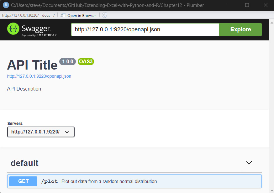
Let’s use a simple analogy: Imagine that you have a restaurant and want to offer a delivery service. You could create a simple website that allows customers to order food online. The website would need to be able to communicate with your restaurant’s kitchen to place orders. In this analogy, the plumber API is like the website, and the R functions are like the restaurant’s kitchen. The plumber API allows you to expose R functions to the outside world so that other applications can communicate with them. Now let’s run the API and see what happens; we do this with the following code: pr_run(root):

Figure 11.8 – plumber GET API

We see that when we run the preceding code, we get a screen back that will allow us to test out the API; so, let’s do just that.

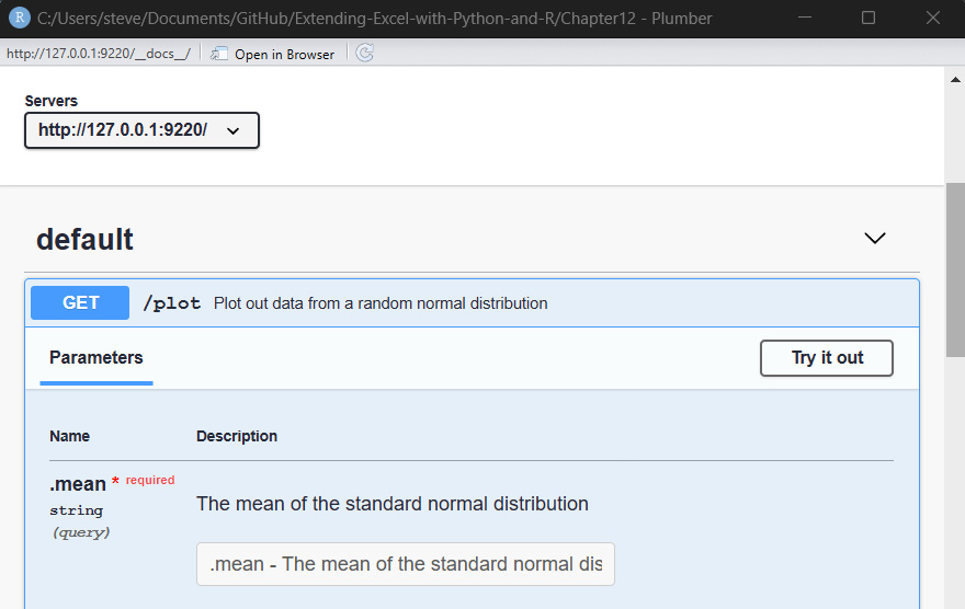
To do that, we can click on the GET button, as this is a GET API call. When we do that, we get the following screen:

Figure 11.9 – Enter arguments for API

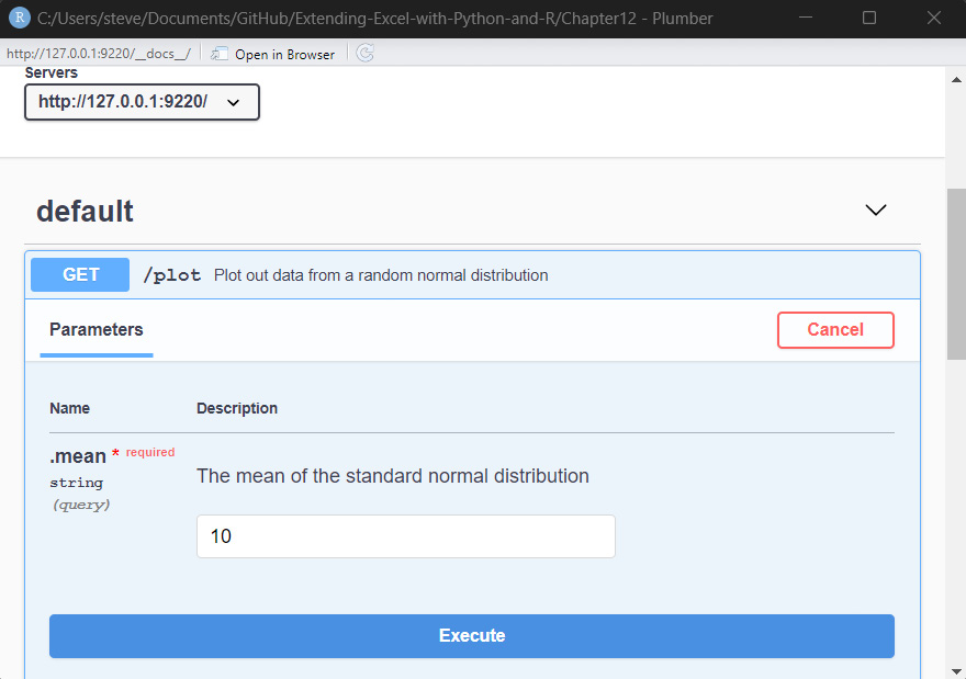
We see that we can enter an argument to the parameter of .mean; let’s enter 10. First, click the Try it out button, and then you can enter a value; then, you can hit Execute, as shown in the following screenshot:

Figure 11.10 – Enter the argument and click Execute

Now, let’s hit that Execute button and check out the output. We get a couple of things; one is the curl request:

curl -X GET "http://127.0.0.1:9220/plot?.mean=10" -H "accept: image/png"

Next, we get the request URL:

http://127.0.0.1:9220/plot?.mean=10

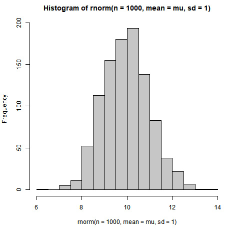
Last but not least, we get the histogram:

Figure 11.11 – The histogram generated by the API call

Now that we have learned how to build and use the API for R, we will learn how to do the same for Python in the next section.