Exercise 2 – network intrusion detection

Applying AI to intrusion detection offers analogous benefits to using AI for malware detection. In the following exercise, we will attempt to detect malicious traffic. For this purpose, we will use support vector machines (SVMs) to construct a model for intrusion detection. SVMs possess several advantages in the realm of intrusion detection systems. They excel in high-dimensional spaces, rendering them suitable for environments where feature spaces are intricate and contain many dimensions. Furthermore, SVMs exhibit resistance to overfitting compared to some alternative algorithms, a trait particularly advantageous when dealing with limited labeled data—a common occurrence in intrusion detection scenarios. Additionally, SVMs demonstrate tolerance to irrelevant features. This is a crucial aspect for intrusion detection, where certain features may hold minimal significance in attack detection. Moreover, they adeptly handle imbalanced datasets, a paramount consideration as intrusion detection datasets often feature limited instances representing attacks.

The dataset employed in this implementation is the NSL-KDD dataset, an updated iteration of the original KDD Cup 1999 dataset. While the KDD Cup 1999 dataset was extensively used to evaluate intrusion detection systems, it presented shortcomings. NSL-KDD rectifies these issues, offering a more realistic depiction of network traffic and a more challenging evaluation environment for intrusion detection systems. Other suitable datasets include UNSW-NB15, CICIDS2017, Kyoto 2006+, and CSE-CIC-IDS2018. The NSL-KDD dataset has an approximate size of 20 MB.

Similarly to the previous exercise, we will begin by importing the requisite libraries. These include standard libraries such as numpy and pandas for numerical operations and data handling, pickle for model serialization, and scikit-learn for preprocessing, model training, and evaluation. Additionally, in this scenario, we import support vector classification (SVC), an implementation of SVM tailored for classification tasks in scikit-learn. This is shown here:

import numpy as np
import pandas as pd
from sklearn.preprocessing import LabelEncoder, StandardScaler
from sklearn.model_selection import train_test_split
from sklearn.svm import SVC
from sklearn.metrics import accuracy_score, classification_report
import pickle

The ensuing source code section entails loading the dataset and conducting preprocessing steps to facilitate compatibility with SVMs and enhance performance. Initially, we will define the columns or features of the dataset. Since the KDDTrain+.txt dataset lacks explicit column headers, we will manually specify the appropriate columns based on the dataset description, the content, and our domain knowledge. Of paramount importance is the label column utilized for classification, distinguishing between normal and abnormal instances. Notably, the dataset constitutes a multiclass classification problem, featuring numerous options for the label column such as normal traffic, DoS attack, and brute force. To accommodate a binary classification problem, we transform the label column, accordingly, categorizing instances as normal or abnormal.

After delineating the columns, we will load the dataset and convert it into a DataFrame using pandas. Subsequently, we will discard columns that are either unusable or that could potentially degrade the model’s performance. For instance, the num_outbound_cmds column holds static values devoid of informational utility. We will then employ the LabelEncoder function to convert categorical variables such as protocol_type, service, and flag into numerical form, thereby enabling compatibility with SVMs.

Lastly, we will convert the label column into binary values, denoted as normal and abnormal, and subsequently transform them into numerical values 0 and 1, respectively, to facilitate SVM usage. Additionally, we will print the count of specific values, such as 50,000 instances of normal traffic and 40,000 of abnormal traffic, for further insight into the dataset’s distribution:

columns =(['duration','protocol_type','service','flag', 
    'src_bytes','dst_bytes','land','wrong_fragment','urgent', 
    'hot','num_failed_logins','logged_in','num_compromised', 
    'root_ shell','su_attempted','num_root', 'num_file_creations', 
    'num_ shells','num_access_files', 'num_outbound_cmds', 
    'is_host_login','is_ guest_login', 'count','srv_count', 
    'serror_rate','srv_serror_rate', 'rerror_rate', 'srv_rerror_rate', 
    'same_srv_rate',  'diff_srv_rate','srv_ diff_host_rate',
    'dst_host_count', 'dst_host_srv_count', 
    'dst_host_same_srv_rate', 'dst_host_diff_srv_rate', 
    'dst_host_same_src_port_rate', 'dst_host_srv_diff_host_rate', 
    'dst_host_serror_rate', 'dst_host_srv_serror_rate',
    'dst_host_rerror_rate', 'dst_host_srv_rerror_rate', 
    'label','difficulty_level']) 
train_data = pd.read_csv(
    'dataset/KDDTrain+.txt', header=None, names=columns)
train_data.drop(
    ['difficulty_level','num_outbound_cmds'],
    axis=1,
    inplace=True)
le = LabelEncoder()
train_data['protocol_type'] = le.fit_transform(
    train_data['protocol_type'])
train_data['service'] = le.fit_transform(
    train_data['service'])
train_data['flag'] = le.fit_transform(train_data['flag'])
train_data['label'] = train_data['label'].apply(
    lambda x: 'normal' if x == 'normal' else 'abnormal')
print(train_data['label'].value_counts())
train_data['label'] = train_data['label'].apply(
    lambda x: 0 if x == 'normal' else 1)

Then in the following code, the dataset is divided into features (X) and labels (y). Subsequently, the dataset undergoes partitioning into training and testing subsets utilizing a 70-30 split. We can omit this step and employ a separate test dataset, such as the KDDTest+ dataset, exclusively for testing purposes, while utilizing the KDDTrain+ dataset solely for model training:

X = train_data.drop(['label'], axis=1)
y = train_data['label']
X_train, X_test, y_train, y_test = train_test_split(
    X, y, test_size=0.30, random_state=40)

Then we will standardize the features using the StandardScaler function for scaling:

scaler = StandardScaler()
X_train = scaler.fit_transform(X_train)
X_test = scaler.transform(X_test)

Next, we will train the model using SVM by initializing an SVM model with a radial basis function (RBF) kernel. Henceforth, the model is trained on the standardized training data. The choice of kernel holds significant importance in SVMs, as different kernels exhibit varying performances and compatibility with diverse techniques and datasets. In our scenario, the rbf kernel demonstrated superior performance to other tested SVM kernels:

svm_model = SVC(kernel='rbf')
svm_model.fit(X_train, y_train)

We will now make predictions on the test set utilizing our trained model. We will print a variety of performance metrics, including accuracy for both the training and testing phases, as well as overall model accuracy. A comprehensive classification report is also generated, encompassing additional metrics such as precision, recall, and F1-score. Finally, we will save our trained model using the pickle library for future use:

y_pred = svm_model.predict(X_test)
print('Training accuracy: ', svm_model.score(X_train, y_train))
print('Testing accuracy: ', svm_model.score(X_test, y_test))
print('SVM Model accuracy: ',
    np.round(accuracy_score(y_test,y_pred),6))
print('Classification Report:\n',
    classification_report(
        y_test,y_pred,target_names=['Normal','Abnormal']
    )
)
pkl_filename = "SVM_model.pkl"
with open(pkl_filename, 'wb') as file:
    pickle.dump(svm_model, file)

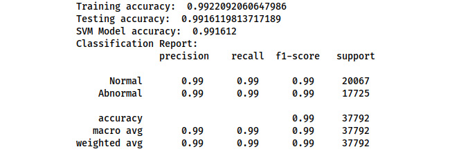
The following is a sample of our program execution:

Figure 7.2 – Execution of SVM model implementation

As shown in the preceding figure, our performance metrics showcase a remarkable 99% accuracy. However, this was attained solely through dataset splitting and not validation on a separate test dataset.

Next, we will provide source code for loading a comprehensive dataset for testing our implementation. It’s crucial to acknowledge that since we have already partitioned the training dataset into train and test subsets, we should exclusively utilize the ensuing test dataset once we remove the train-test partitioning code. Failure to do so may adversely impact the model’s performance.

print('Starting Testing Process using the Test Dataset....')
test_data = pd.read_csv('dataset/KDDTest+.txt',
    header=None, names=columns)
test_data.drop(['difficulty_level', 'num_outbound_cmds'],
    axis=1, inplace=True)
le = LabelEncoder()
test_data['protocol_type'] = le.fit_transform(
    test_data['protocol_type'])
test_data['service'] = le.fit_transform(test_data['service'])
test_data['flag'] = le.fit_transform(test_data['flag'])
test_data['label'] = test_data['label'].apply(
    lambda x: 0 if x == 'normal' else 1)
X_test = test_data.drop(['label'], axis=1)
y_test = test_data['label']
X_test = scaler.transform(X_test)
y_pred = svm_model.predict(X_test)
print('Testing Phase accuracy: ', accuracy_score(y_test, y_pred))
print('SVM Model accuracy: ', accuracy_score(y_test, y_pred))
print('Classification Report:\n',
    classification_report(y_test, y_pred,
        target_names=["Normal", "Abnormal"]))

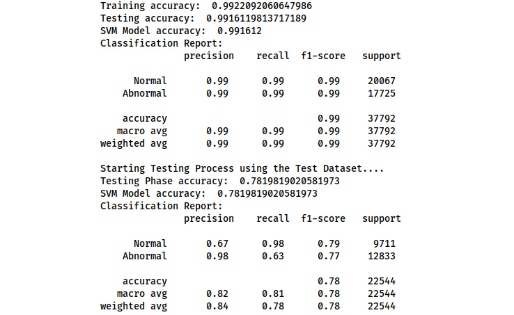
Here is the performance of the implementation using the test dataset:

Figure 7.3 – Execution of SVM model implementation

This highlights the performance of our model in real-world scenarios, showcasing an accuracy of approximately 80%. The observed deviation in performance signals the presence of overfitting, a common occurrence under such circumstances. Notably, feature selection was not conducted on the dataset, allowing certain features to contribute to overfitting. Additionally, the dataset itself is relatively small. Using an RBF kernel, which is susceptible to overfitting on small datasets, further exacerbates this issue.

Moreover, no fine-tuning was performed on the kernel itself, compounding the problem. However, in the final implementation, these issues will be addressed. By integrating feature selection alongside a different algorithm, such as recurrent neural networks (RNNs), and refining the model, we can anticipate achieving a performance exceeding 95% in real-world environments.

Deep learning techniques, notably neural networks, can discern intricate patterns and relationships in data. They excel in learning from large datasets and are adaptable to structured and unstructured data. Neural networks have consistently demonstrated high performance in the domain of intrusion detection. Convolutional neural networks (CNNs) are particularly effective in image-based intrusion detection. In contrast, RNNs excel in handling sequential data.