Search icon CANCEL
Subscription
0
Cart icon
Your Cart (0 item)
Close icon
You have no products in your basket yet
Arrow left icon
Explore Products
Best Sellers
New Releases
Books
Videos
Audiobooks
Learning Hub
Free Learning
Arrow right icon
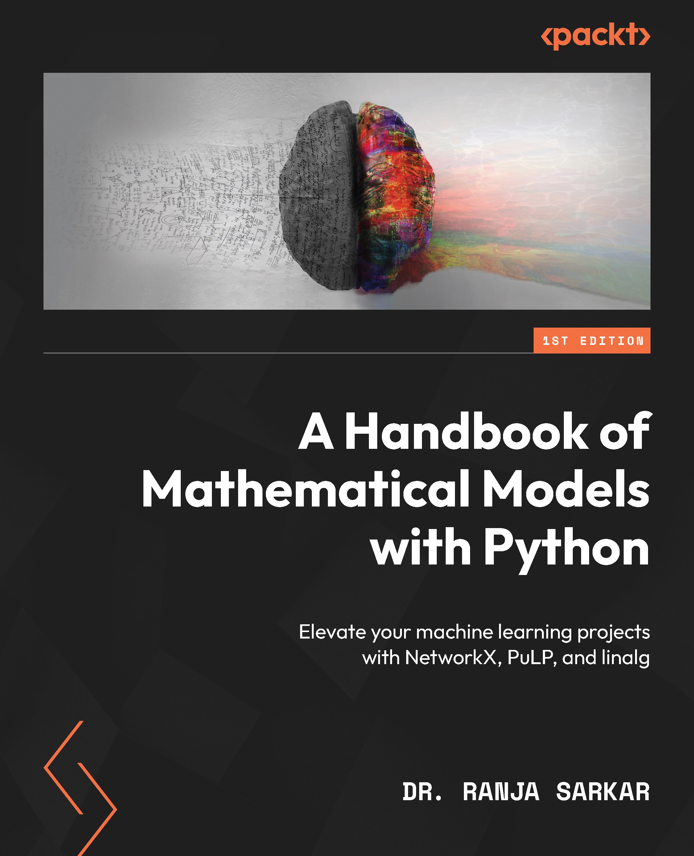
A Handbook of Mathematical Models with Python

A Handbook of Mathematical Models with Python: Elevate your machine learning projects with NetworkX, PuLP, and linalg

eBook
€8.99 €29.99
Paperback
€37.99
Subscription
Free Trial
Renews at €18.99p/m

What do you get with eBook?

Product feature icon Instant access to your Digital eBook purchase
Product feature icon Download this book in EPUB and PDF formats
Product feature icon Access this title in our online reader with advanced features
Product feature icon DRM FREE - Read whenever, wherever and however you want
Product feature icon AI Assistant (beta) to help accelerate your learning
OR
Modal Close icon
Payment Processing...
tick Completed

Billing Address

Table of content icon View table of contents Preview book icon Preview Book

A Handbook of Mathematical Models with Python

Introduction to Mathematical Modeling

There is a great deal of interesting work happening in data sciences, especially in the realms of Machine Learning (ML) and Deep Learning (DL), and they are popular for good reason. However, the more tried and tested old-timer, mathematical modeling, is not much talked about. Mathematical modeling methods are no less relevant and are complementary to ML. To create successful data products that solve real business problems, we must often deploy the whole breadth of available mathematical tools, far beyond ML.

A model is a simplified representation of a real system and captures the essence of the system. A mathematical model uses variables, operators, functions, equations, and equalities. Under the hood of mathematical models, there are first-principle models based on physical laws, stochastic models based on distributions, averages, and empirical models based on patterns or historical data. Based on the particular type of modeling, qualitative or quantitative recommendations can be made for the system under consideration. A mathematical model facilitates design and prototyping and substantiates decisions. To formulate a mathematical model, one needs the input and output, the constants and variables, the domain and boundary, or initial conditions and constraints. The solution can be analytic or numerical; in either case, it determines the typical behavior and critical parameters of the system, trends, dependency, and operating regimes. Systems can be deterministic, wherein we know the cause-effect relationship, or they may be stochastic, involving probability distributions.

A few mature tools in mathematical modeling are in the following areas:

  • Mathematical optimization
  • Signal processing
  • Control theory

We will explore these mathematical modeling approaches in the following sections. A narrow focus on ML misses out on many relevant features of pure mathematical optimization in many use cases. Successful solutions across disparate domains blend the new world of ML with classical mathematical modeling techniques. For example, one can combine state-space modeling methods with ML to infer unobserved parameters of systems in a parameter estimation problem.

Mathematical optimization

A branch of applied mathematics is mathematical optimization, popularly known as mathematical programming. It finds applications in fields such as manufacturing, inventory control, scheduling, networks, economics, engineering, and financial portfolio allocation. Almost any classification, regression, or clustering problem can be cast as an optimization problem. Some problems are static, while some are dynamic, wherein the values of system variables change over time.

Understanding the problem

Mathematical optimization is basically choosing inputs from a set of allowed options to obtain the optimized or best possible output in a given problem. There are variables, which are essentially the decisions we have to make; constraints, which are the business rules we have to adhere to; and objectives, which are the business goals we are aiming to achieve by representing the real-world business problem as an optimization problem. For example, a hospital’s business problem is equipment and facility capacity planning. Medical equipment including beds and testing kits comprise the decision variables in this case; constraints are conventional and crisis capacity levels and regulations; and finally, the objective is to maximize resource utilization and service performance and minimize operating costs at the same time.

The most basic optimization problem consists of an objective function or cost function, which is the output value we try to optimize, in other words, maximize or minimize. The inputs are variables that can be controlled. Variables can be either discrete or continuous. The scale of a problem is pretty much determined by the dimensionality, that is, the number of scalar variables (also called decision variables) on which the search is performed. Constraints or equations place limits on how big or small some variables can get. Some problems have constraints, which can be equality or inequality constraints, while some problems do not have them at all, which implies the unbounded optimization of the function.

A linear programming problem is an optimization problem wherein the objective function and all constraints are linear, that is, the variables have only first-order terms. It was linear programming that led to the development of optimization in the 1940s. If either the function or one or more constraint(s) is non-linear, then we have a non-linear programming problem. For example, optimizing smooth (well-defined gradient, continuous) functions is easier. Knowing the problem type enables the selection of the right tool to solve it.

Formulation of the problem

The general formulation of a mathematical problem with an objective function f(x) represents questions in terms of variables and constraints. A typical form is as follows:

Minimize f ( such that where i = 1, 2, ...., m

The nature of variables and constraints can be quite diverse. The variables may be discrete, continuous, or sets (groups), and the constraints may be deterministic or stochastic. The objective function may also include dynamic aspects.

Sometimes we are interested in finding the global optimum point without any constraints or restrictions on the region in space. Such problems are unconstrained optimization problems. At other times, we have to solve problems subject to certain constraints, such as restrictions on control variables. For example, in the preceding case, we might have to minimize the function subject to (. These are constrained optimization problems.

Example 1:

Let us have multiple (inequalities) constraints with two variables, x and y, as follows:

2x + 3y ≤ 34

3x + 5y ≤ 54

0 ≤ x, y

A graphical optimization would be an overlap (dark region) of the graphs, shown in Figure 1.1. Here the constraints are linear, and therefore, the maximum and minimum must lie on the boundary. And it is most likely that the optimum solution occurs at one of the three specified points. With non-linear constraints, the optimum occurs either at the boundaries or between them. In unconstrained optimization, either the function has no boundaries, or if it has, they are soft.

Figure 1.1: Graphical representation of linear constrained optimization

Figure 1.1: Graphical representation of linear constrained optimization

Typical constraints in business problems involve time, money, and resources while attempting to maximize an objective function. The constraints are more particular to the use case at hand while minimizing an objective function. Suppose in the preceding problem the objective function is linear, such as f(x, y) = 20x + 35y, and the optimum is found out from the slope of the function. If f(x, y) takes a value, the value becomes a boundary, and the constraint plus the boundary make a linear constraint.

With linear constraints, the overlap region is considered to be feasible. Non-linear constraints can be very difficult to visualize as a distorted x-y plane makes it almost impossible to graph the feasible region.

Example 2:

In non-linear constrained optimization, the first step is to start on the boundary of the feasible region. To minimize the objective function, the vector direction should be chosen so that it decreases the function and stays in the feasible region. If the dot product of the gradient (slope) of the objective function with the vector itself is negative at a point on the boundary, then the vector is said to be moving in the descent direction. Also, a vector that does not violate the constraints is said to move in a feasible direction.

Figure 1.2: Feasible direction in non-linear constrained optimization

Figure 1.2: Feasible direction in non-linear constrained optimization

The constraint equation on the boundary is g(x) =0, shown in Figure 1.2. A feasible vector cannot cause the value of g(x) to increase. It must either remain zero or decrease. If the dot product of the gradient of the constraint with the vector itself is negative or zero at the point, then the vector is said to be moving in a feasible direction. For example, say we have the following objective function:

Minimize

And the initial point (4, 2 on a single constraint:

Where and are the variables, in general, standing for a matrix or array. The vector <-1, 0> is in both descent and feasible directions. Since the initial point is randomly chosen, there is a good chance that the overlap between the set of all feasible vectors and the set of all descent vectors is large. However, as we approach the minimum, the overlap gets smaller, and at the minimum or optimum point, there is no overlap at all. At the optimum, one cannot minimize the objective function further without violating the constraint. We know we have reached the optimum when the dot product of the two gradients is negative, and the two vectors have a matrix determinant equal to zero.

Another possibility is that the optimum occurs in the interior of the feasible region rather than on the boundary. In such a case, the gradient of the objective function will be zero at that point. The concavity (non-convexity) of the point is determined by the eigenvalues of Hessian (second differential) of the function.

In optimization problems where the objective function is noisy or its gradient is computed numerically as the gradient is not given (complex boundary value problems, for instance), errors are induced. Even if the objective functions themselves are not noisy, gradient-based optimization may turn out to be noisy. There are different optimizers available as library functions with Scientific Python, or scipy for short, to solve such optimization problems, and we will learn about a few of them in the following chapters. Now that we have learned about the concepts of mathematical optimization, we shall explore another concept in mathematical modeling, which is signal processing.

Signal processing

Another branch of applied mathematics is signal processing, which finds its application in the engineering field, focusing on analyzing and processing signals such as sound, images, scientific measurements, and filtering out noise. Signal processing deals with the transformation of a signal from time-series to hyper-spectral images, which are obtained from different electromagnetic measurements. Classic transformations of signals such as spectrograms and wavelets are often used with ML techniques. Such representations can also be used as inputs to deep neural networks. The Kalman filter is one classic signal processing filter that uses a series of measurements over time to produce estimates of unknown variables.

Understanding the problem

A signal is a function of a continuous variable, such as time or space. An analog signal is transformed into a digital signal by sampling it at specified intervals of time called the sampling period, the inverse of which is the sampling rate (per second or Hertz). The sampling rate has to be at least twice as high as the maximum frequency of the analog signal. It establishes a sufficient condition that permits a discrete sequence of samples to encapsulate all the information from a continuous time signal into a discrete time signal.

Figure 1.3: 60 kHz sinusoidal (Hann-windowed) tone burst in the time domain and frequency domain of the signal

Figure 1.3: 60 kHz sinusoidal (Hann-windowed) tone burst in the time domain and frequency domain of the signal

The frequency domain representation of a signal is done with the Discrete Fourier Transform (DFT). The Fast Fourier Transform (FFT) is an efficient computation method of DFT. FFT is rarely applied over the entire signal (speech signal, for example) at once but rather in frames due to the stochastic nature of the signal, an example of which is illustrated in Figure 1.3. FFT is available as a library function with scipy for the computation of the frequencies of each frame. A type of Fourier transform called the Short-time Fourier Transform (STFT) is typically applied on each individual frame.

Formulation of the problem

It is clear that Discrete-Time Signal Processing (DSP) is meant for sampled signals and establishes a mathematical basis for DSP, which is essentially analyzing and modifying a signal to improve (or optimize) its efficiency or performance. By using DFT, a discrete sequence can be represented as its equivalent frequency ‘ domain. The linearity property of the Fourier transform yields two signals, and :

Where and are the Fourier transforms of and respectively, a concept often used in the filtering of signals, which is the transformation of the time domain to the frequency domain. The duality property of the Fourier transform is useful as it enables solving complex ones that otherwise would be difficult to compute directly. It yields that if x has a Fourier transform , then one can form a new function of time that has a functional form of the transformation, for example:

A time shift affects the frequency, and a frequency shift affects the time of the functions. Let us take an example of a spectrogram to understand DSP.

A spectrogram displays the spectrum of frequencies of a waveform over time and is extensively used in the fields of music and speech processing and radars. It is generated by an optical spectrometer, a Fourier transform, or a wavelet transform and is usually depicted as a heat map wherein the strength or intensity of the signal changes with the color (brightness). To generate a spectrogram, a time-domain signal is divided into chunks of equal lengths that usually overlap, and FFT is applied to each chunk for the calculation of the frequency range. The spectrogram is a plot or graph of the spectrum on each segment or FFT frame, as a frequency versus a time image (or a 3D surface), shown in Figure 1.4, and the third dimension (represented by the color bar) indicates the amplitude of a particular frequency at a particular time. This process corresponds to the computation of the squared magnitude of STFT of the signal.

Figure 1.4: Spectrogram

Figure 1.4: Spectrogram

Spectrograms can be used to identify characteristics of non-stationary or non-linear signals as a collection of time-frequency analyses. The parameters in a spectrogram typically are frame count (number of FFTs making it up), frequency range (minimum and maximum), FFT spacing, and FFT width (width of time each FFT represents).

Spectrograms are used with recurrent neural networks (RNNs) in speech recognition, as a primary example. We learned about how digital signals are free (well, almost) of noise and less distorted in this sub-section, and in the next, we are going to explore control theory, another mathematical modeling technique widely used in industrial processes. Control theory is, in general, useful whenever feedback happens in either regulator or servo mechanisms, for example, navigation systems and industrial production processes.

Control theory

A branch of mathematics and engineering is control theory, which found its use in social sciences as well, such as economics and psychology. It deals with the behavior or evolution of dynamical systems. It is particularly useful when the dynamics of a system are not arbitrary, that is, we understand the physics of the system. The objective of control is to develop a model from measured data. This model is a mathematical description of inputs applied to drive a system to a desired state, minimizing any delay or error simultaneously and ensuring a level of stability.

The behavior of a dynamical system is influenced by a feedback loop – a controller manipulates the system inputs to obtain the desired effect on the output. An error-controlled regulation is typically carried out with a proportional-integral-derivative (PID) controller, and as the name suggests, the signal is derived from a weighted sum, integral, and derivative of the error signal. The error, which is the difference between the actual and the desired output, is applied as feedback to the input. The standard terminology for a system is a process, and for a controlled variable is a process variable (PV), and the objective remains the reduction of the deviation error. Using a negative feedback loop, a measurement of PV (E in Figure 1.5) is deducted from a desired value S (set point or SP) to estimate an error (SP minus PV) in the system, which is used by a regulator R (Figure 1.5) to reduce the gap between the measured value and desired value. The error may be introduced into the system T as a disturbance D, as shown in the closed loop (Figure 1.5) of a controller.

Figure 1.5: Negative feedback controller

Figure 1.5: Negative feedback controller

Control theory can be linear as well as non-linear. Linear control theory is applied to devices obeying the superposition principle, meaning the output is roughly proportional to the input. Such (close to ideal) systems are tractable by frequency domain mathematical techniques such as Laplace transform, Fourier transform, and the Nyquist stability criterion. Non-linear control theory, on the other hand, applies to real-world systems that do not obey the superposition principle. Such systems are often governed by non-linear differential equations and analyzed using numerical methods. Non-linear systems are studied numerically using simulating operations using a simulation language that mirrors the system processes. However, if solutions in the vicinity of a stable or equilibrium point are only of interest, non-linear control systems can be linearized into approximations using perturbation techniques.

Understanding the problem

Mathematical techniques are served in either the frequency domain or time domain for analyzing control systems. The state variables in a frequency domain, representing the system’s input, output, and feedback, are functions of frequency. The transfer function, system function, or network function is a mathematical model of the relationship between the input and output, on the basis of differential equations governing or describing the system. The input and transfer functions are converted from functions of time to functions of frequency by a mathematical transformation. In this domain, the differential equations are replaced by algebraic equations, which are simpler to solve. The state variables in a time domain are functions of time, and the system is described by one or more differential equations.

Time domain techniques are used to explore and analyze real non-linear systems because frequency domain techniques can only be used to study (ideal) linear systems. Although the equations for non-linear systems are difficult to solve, computer simulation methods have made their analyses commonplace. A critical application of the control loop is in industrial process control systems design, as shown in Figure 1.6.

Figure 1.6: Industrial control showing continuously modulated process flow

Figure 1.6: Industrial control showing continuously modulated process flow

The building block of industrial processes is the control loop, which consists of all elements to measure and control a process value at a desired SP in the presence of perturbances. The controller may be an isolated piece of hardware or, within a large distributed control system, a programmable logic controller (PLC) system and SP inputs can be manually set or cascaded from another source. The green text in Figure 1.6 are tags that describe the function and identify a component and are unique (strings) within a plant representing the equipment components or elements. An associated sensor essentially captures the data of such tags.

Formulation of the problem

Modern control theory utilizes state-space methods (time-domain representation), unlike classical control theory, which uses transform methods (frequency-domain representation) such as the Laplace transform, which encodes all system information. In the state-space approach, a mathematical model is a set of first-order differential equations governing the related set of input, output, and state variables of the system. These variables are expressed as vectors, and the differential equations have a matrix format, which is more convenient to tackle. On the contrary, algebraic equations representing the behavior of a linear dynamical system are written in matrix form.

The state-space approach is not limited to linear systems and provides a convenient and compact way of modeling and analyzing mostly non-linear systems with multiple inputs and outputs. State space refers to a space whose axes are state variables, and the system state is expressed as a vector within that space.

A plant or process is the part of the system that is controlled, and the controller (or simply filter) makes up the rest. Inputs to the process have an effect on the outputs, and the effect is measured with sensors and processed by the controller. The control signal is fed back to the input, thus closing the loop. Such a typical architecture is the PID controller, which is by and large the most used industrial design, shown in Figure 1.7. It calculates an error value e(t) continuously, the error being the difference between the desired SP and measured PV, and applies a correction on the basis of proportional, integral, and derivative terms.

Figure 1.7: u(t) is the control signal sent to the system, e(t) = r(t) – y(t) is the error

Figure 1.7: u(t) is the control signal sent to the system, e(t) = r(t) – y(t) is the error

When such a process is monitored by multiple controllers, it becomes a distributed control system with a decentralized control loop. Decentralization is useful as it helps the control systems to operate over a large area while interaction happens through communication channels.

Some of the main control techniques extensively used in industries include adaptive control, hierarchical control, optimal control, robust control, and stochastic control. Apart from these, intelligent control uses artificial intelligence (AI) and ML approaches such as fuzzy logic, neural networks, and so on to control a dynamic system. Industry 4.0 is revolutionizing the way manufacturers are integrating AI into their operations and production facilities.

Summary

In this chapter, we introduced the concepts of mathematical modeling via the important areas it is largely implemented in or applied to, such as optimization, signal processing, control systems, and control engineering. Mathematical modeling or mathematical programming is the art of transforming a problem into a clear mathematical formulation. Its subsequent algorithmic implementation generates actionable insights and helps build further knowledge about the domain.

The chapter helped us learn the formulation of a mathematical optimization problem in order to arrive at an optimal solution, the formulation being dependent on the domain we intend to investigate. A mathematical optimization model is like a digital twin of a real-world business scenario. It mirrors the business landscape in a strictly mathematical and programming setup, and such an environment becomes particularly relevant for the interpretability of business processes to support high-stake decisions.

In the next chapter, we will find out how mathematical models emphasize the importance of both data and domain knowledge. Additionally, we will learn how ML models can be cast as optimization problems.

Left arrow icon Right arrow icon
Download code icon Download Code

Key benefits

  • Gain a profound understanding of various mathematical models that can be integrated with machine learning
  • Learn how to implement optimization algorithms to tune machine learning models
  • Build optimal solutions for practical use cases
  • Purchase of the print or Kindle book includes a free PDF eBook

Description

Mathematical modeling is the art of transforming a business problem into a well-defined mathematical formulation. Its emphasis on interpretability is particularly crucial when deploying a model to support high-stake decisions in sensitive sectors like pharmaceuticals and healthcare. Through this book, you’ll gain a firm grasp of the foundational mathematics underpinning various machine learning algorithms. Equipped with this knowledge, you can modify algorithms to suit your business problem. Starting with the basic theory and concepts of mathematical modeling, you’ll explore an array of mathematical tools that will empower you to extract insights and understand the data better, which in turn will aid in making optimal, data-driven decisions. The book allows you to explore mathematical optimization and its wide range of applications, and concludes by highlighting the synergetic value derived from blending mathematical models with machine learning. Ultimately, you’ll be able to apply everything you’ve learned to choose the most fitting methodologies for the business problems you encounter.

Who is this book for?

If you are a budding data scientist seeking to augment your journey with mathematics, this book is for you. Researchers and R&D scientists will also be able to harness the concepts covered to their full potential. To make the best use of this book, a background in linear algebra, differential equations, basics of statistics, data types, data structures, and numerical algorithms will be useful.

What you will learn

  • Understand core concepts of mathematical models and their relevance in solving problems
  • Explore various approaches to modeling and learning using Python
  • Work with tested mathematical tools to gather meaningful insights
  • Blend mathematical modeling with machine learning to find optimal solutions to business problems
  • Optimize ML models built with business data, apply them to understand their impact on the business, and address critical questions
  • Apply mathematical optimization for data-scarce problems where the objective and constraints are known

Product Details

Country selected
Publication date, Length, Edition, Language, ISBN-13
Publication date : Aug 30, 2023
Length: 144 pages
Edition : 1st
Language : English
ISBN-13 : 9781804617069
Category :

What do you get with eBook?

Product feature icon Instant access to your Digital eBook purchase
Product feature icon Download this book in EPUB and PDF formats
Product feature icon Access this title in our online reader with advanced features
Product feature icon DRM FREE - Read whenever, wherever and however you want
Product feature icon AI Assistant (beta) to help accelerate your learning
OR
Modal Close icon
Payment Processing...
tick Completed

Billing Address

Product Details

Publication date : Aug 30, 2023
Length: 144 pages
Edition : 1st
Language : English
ISBN-13 : 9781804617069
Category :

Packt Subscriptions

See our plans and pricing
Modal Close icon
€18.99 billed monthly
Feature tick icon Unlimited access to Packt's library of 7,000+ practical books and videos
Feature tick icon Constantly refreshed with 50+ new titles a month
Feature tick icon Exclusive Early access to books as they're written
Feature tick icon Solve problems while you work with advanced search and reference features
Feature tick icon Offline reading on the mobile app
Feature tick icon Simple pricing, no contract
€189.99 billed annually
Feature tick icon Unlimited access to Packt's library of 7,000+ practical books and videos
Feature tick icon Constantly refreshed with 50+ new titles a month
Feature tick icon Exclusive Early access to books as they're written
Feature tick icon Solve problems while you work with advanced search and reference features
Feature tick icon Offline reading on the mobile app
Feature tick icon Choose a DRM-free eBook or Video every month to keep
Feature tick icon PLUS own as many other DRM-free eBooks or Videos as you like for just €5 each
Feature tick icon Exclusive print discounts
€264.99 billed in 18 months
Feature tick icon Unlimited access to Packt's library of 7,000+ practical books and videos
Feature tick icon Constantly refreshed with 50+ new titles a month
Feature tick icon Exclusive Early access to books as they're written
Feature tick icon Solve problems while you work with advanced search and reference features
Feature tick icon Offline reading on the mobile app
Feature tick icon Choose a DRM-free eBook or Video every month to keep
Feature tick icon PLUS own as many other DRM-free eBooks or Videos as you like for just €5 each
Feature tick icon Exclusive print discounts

Frequently bought together


Stars icon
Total 105.97
Building Statistical Models in Python
€37.99
A Handbook of Mathematical Models with Python
€37.99
Causal Inference and Discovery in Python
€29.99
Total 105.97 Stars icon
Banner background image

Table of Contents

15 Chapters
Part 1:Mathematical Modeling Chevron down icon Chevron up icon
Chapter 1: Introduction to Mathematical Modeling Chevron down icon Chevron up icon
Chapter 2: Machine Learning vis-à-vis Mathematical Modeling Chevron down icon Chevron up icon
Part 2:Mathematical Tools Chevron down icon Chevron up icon
Chapter 3: Principal Component Analysis Chevron down icon Chevron up icon
Chapter 4: Gradient Descent Chevron down icon Chevron up icon
Chapter 5: Support Vector Machine Chevron down icon Chevron up icon
Chapter 6: Graph Theory Chevron down icon Chevron up icon
Chapter 7: Kalman Filter Chevron down icon Chevron up icon
Chapter 8: Markov Chain Chevron down icon Chevron up icon
Part 3:Mathematical Optimization Chevron down icon Chevron up icon
Chapter 9: Exploring Optimization Techniques Chevron down icon Chevron up icon
Chapter 10: Optimization Techniques for Machine Learning Chevron down icon Chevron up icon
Index Chevron down icon Chevron up icon
Other Books You May Enjoy Chevron down icon Chevron up icon

Customer reviews

Top Reviews
Rating distribution
Full star icon Full star icon Full star icon Full star icon Half star icon 4.1
(7 Ratings)
5 star 57.1%
4 star 28.6%
3 star 0%
2 star 0%
1 star 14.3%
Filter icon Filter
Top Reviews

Filter reviews by


Om S Sep 10, 2023
Full star icon Full star icon Full star icon Full star icon Full star icon 5
The book begins by introducing the concept of mathematical modeling and its significance in solving practical problems. It then takes readers through a journey of various mathematical models and demonstrates how Python can be used as a tool to implement and work with these models effectively.One of the book's strengths is its emphasis on hands-on learning. It provides practical examples and exercises that allow readers to apply mathematical models to real-life scenarios. This hands-on approach not only enhances understanding but also equips readers with valuable problem-solving skills.Throughout the book, readers will explore a wide range of mathematical concepts and their applications, from basic principles to more advanced topics. The book also covers optimization techniques, which are essential for finding the best solutions to complex problems.Whether you are a student looking to learn mathematical modeling or a professional seeking to apply these techniques in your work, this book provides a solid foundation. It is written in a clear and accessible manner, making it suitable for readers with various levels of mathematical and programming expertise.In conclusion, "A Handbook of Mathematical Models with Python" is a practical and user-friendly guide that demystifies mathematical modeling and demonstrates how to implement it using Python. It is a valuable resource for anyone looking to enhance their problem-solving skills and apply mathematics to real-world challenges.
Amazon Verified review Amazon
Kumar Abhishek Dec 30, 2023
Full star icon Full star icon Full star icon Full star icon Full star icon 5
This book is a concise, 100-page guide that provides a quick yet insightful overview of mathematical models and their connection to machine learning. As a senior machine learning engineer, I found this book to be a helpful introduction for those who are beginning their journey in data science or those who feel lacking in math knowledge. It effectively links fundamental mathematical concepts with Python applications in machine learning, offering practical examples and use cases. While the book is an excellent starting point for understanding the interplay between math and machine learning, it's important to note that it doesn't delve into deep technical details. For readers seeking in-depth mathematical explanations, I would recommend more mathematically intensive books. Nevertheless, for a clear, introductory understanding of how mathematics underpins machine learning algorithms, Dr. Sarkar's book is a valuable and accessible resource.
Amazon Verified review Amazon
Greg Phillips Feb 06, 2024
Full star icon Full star icon Full star icon Full star icon Full star icon 5
This is an excellent book to get you started on the path towards a better understanding of the math underpinning Machine Learning as implemented with Python. Reading is time well spent.
Amazon Verified review Amazon
Rahul Bahadur Oct 09, 2023
Full star icon Full star icon Full star icon Full star icon Full star icon 5
While most ML books delve straight into applications, this book describes, in detail, what goes on mathematically under the hood - without being overwhelming. It starts with describing some of the most common algorithms that any Data Scientist/Statistician uses (like PCA, SVM, Linear regression, neural-nets) and their applications. Later it also describes MCMC chains, Kalman filters etc. along with graph optimizations (travelling salesperson).One of the most common mistake that a data scientist does is treating everything as an ML prediction problem. This book talks about scenarios where one would apply linear programming (PuLP), network modelling etc. to come up with the correct solution.Each chapter has plenty of follow along example in python using commonly available libraries. The author also mentions a lot of great online resources if you want to delve further into any topic.All in all this is a great quick read if you are looking to refresh your understanding or even starting to explore what all methods should exists in your problem solving toolbox.
Amazon Verified review Amazon
H2N Nov 16, 2023
Full star icon Full star icon Full star icon Full star icon Empty star icon 4
This book is an essential resource for data scientists and R&D professionals, offering a practical approach to mathematical modeling in Python. It's ideal for those familiar with differential equations, linear algebra, and statistics, blending machine learning with classical models. Covering PCA, Gradient Descent, SVMs, and more, it excels in explaining data classification and reduction. Additionally, it touches on Graph Theory, Kalman Filter, and Markov Chains, culminating in strategies for optimizing machine learning models. While concise, it leaves readers anticipating a more in-depth exploration in future editions.
Amazon Verified review Amazon
Get free access to Packt library with over 7500+ books and video courses for 7 days!
Start Free Trial

FAQs

How do I buy and download an eBook? Chevron down icon Chevron up icon

Where there is an eBook version of a title available, you can buy it from the book details for that title. Add either the standalone eBook or the eBook and print book bundle to your shopping cart. Your eBook will show in your cart as a product on its own. After completing checkout and payment in the normal way, you will receive your receipt on the screen containing a link to a personalised PDF download file. This link will remain active for 30 days. You can download backup copies of the file by logging in to your account at any time.

If you already have Adobe reader installed, then clicking on the link will download and open the PDF file directly. If you don't, then save the PDF file on your machine and download the Reader to view it.

Please Note: Packt eBooks are non-returnable and non-refundable.

Packt eBook and Licensing When you buy an eBook from Packt Publishing, completing your purchase means you accept the terms of our licence agreement. Please read the full text of the agreement. In it we have tried to balance the need for the ebook to be usable for you the reader with our needs to protect the rights of us as Publishers and of our authors. In summary, the agreement says:

  • You may make copies of your eBook for your own use onto any machine
  • You may not pass copies of the eBook on to anyone else
How can I make a purchase on your website? Chevron down icon Chevron up icon

If you want to purchase a video course, eBook or Bundle (Print+eBook) please follow below steps:

  1. Register on our website using your email address and the password.
  2. Search for the title by name or ISBN using the search option.
  3. Select the title you want to purchase.
  4. Choose the format you wish to purchase the title in; if you order the Print Book, you get a free eBook copy of the same title. 
  5. Proceed with the checkout process (payment to be made using Credit Card, Debit Cart, or PayPal)
Where can I access support around an eBook? Chevron down icon Chevron up icon
  • If you experience a problem with using or installing Adobe Reader, the contact Adobe directly.
  • To view the errata for the book, see www.packtpub.com/support and view the pages for the title you have.
  • To view your account details or to download a new copy of the book go to www.packtpub.com/account
  • To contact us directly if a problem is not resolved, use www.packtpub.com/contact-us
What eBook formats do Packt support? Chevron down icon Chevron up icon

Our eBooks are currently available in a variety of formats such as PDF and ePubs. In the future, this may well change with trends and development in technology, but please note that our PDFs are not Adobe eBook Reader format, which has greater restrictions on security.

You will need to use Adobe Reader v9 or later in order to read Packt's PDF eBooks.

What are the benefits of eBooks? Chevron down icon Chevron up icon
  • You can get the information you need immediately
  • You can easily take them with you on a laptop
  • You can download them an unlimited number of times
  • You can print them out
  • They are copy-paste enabled
  • They are searchable
  • There is no password protection
  • They are lower price than print
  • They save resources and space
What is an eBook? Chevron down icon Chevron up icon

Packt eBooks are a complete electronic version of the print edition, available in PDF and ePub formats. Every piece of content down to the page numbering is the same. Because we save the costs of printing and shipping the book to you, we are able to offer eBooks at a lower cost than print editions.

When you have purchased an eBook, simply login to your account and click on the link in Your Download Area. We recommend you saving the file to your hard drive before opening it.

For optimal viewing of our eBooks, we recommend you download and install the free Adobe Reader version 9.