Chapter 7. Introduction to Computer Vision
In the previous chapter, we implemented a battery-operated portable Pi time-lapse box and a stop motion recording system. In this chapter, we will cover the basics of computer vision with Pi using the OpenCV library. OpenCV is a simple yet powerful tool for any computer vision enthusiast. One can learn about computer vision in an easy way by writing OpenCV programs in Python. Using a Raspberry Pi computer and Python for OpenCV programming is one of the best ways to start your journey in the world of computer vision. We will cover the following topics in detail in this chapter:
- Introducing computer vision
- Introducing OpenCV
- Setting up Pi for computer vision and NumPy
- Image basics in OpenCV
- Webcam video processing with OpenCV
- Arithmetic and logical operations on images
- Colorspace and the conversion of colorspace
- Object tracking based on colors
Introducing Computer Vision
Computer vision is an area of computer science, mathematics, and electrical engineering. It includes ways to acquire, process, analyze, and understand images and videos from the real world in order to mimic human vision. Also, unlike human vision, computer vision can also be used to analyze and process depth and infrared images. Computer vision is also concerned with the theory of information extraction from images and videos. A computer vision system can accept different forms of data as an input, including—but not limited to—images, image sequences, and videos that can be streamed from multiple sources to further process and extract useful information from it for decision making. Artificial intelligence and computer vision share many topics, such as image processing, pattern recognition, and machine learning techniques.
Introducing OpenCV
OpenCV (short for Open Source Computer Vision) is a library of programming functions for computer vision. It was initially developed by the Intel Russia research center in Nizhny Novgorod, and it is currently maintained by Itseez.
Note
You can read more about Itseez at http://itseez.com/.
This is a cross-platform library, which means that it can be implemented and operated on different operating systems. It focuses mainly on image and video processing. In addition to this, it has several GUI and event handling features for the user's convenience.
OpenCV was released under a Berkeley Software Distribution (BSD) license, and hence, it is free for both academic and commercial use. It has interfaces for popular programming languages, such as C/C++, Python, and Java, and it runs on a variety of operating systems, including Windows, Android, and Unix-like operating systems.
Note
You can explore the OpenCV homepage, www.opencv.org, for further details.
OpenCV was initially an Intel Research initiative to develop tools to analyze images. The following is the timeline of OpenCV in brief:
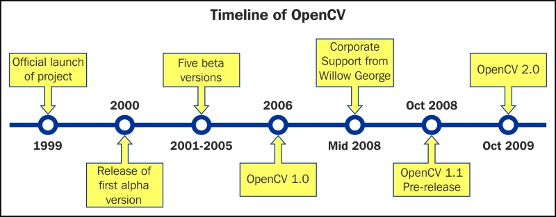
In August 2012, support for OpenCV was taken over by a nonprofit foundation, www.OpenCV.org, which is currently developing it further. It also maintains a developer and user site for OpenCV.
Note
At the time of writing this, the stable version of OpenCV is 2.4.10. Version 3.0 Beta is also available.
Setting up Pi for Computer Vision
Make sure that you have a working, wired Internet connection with reasonable speed for this activity. Now, let's prepare our Pi for computer vision:
- Connect your Pi to the Internet through Ethernet or a Wi-Fi USB dongle.
- Run the following command to restart the networking service:
sudo service networking restart - Make sure that Raspberry Pi is connected to the Internet by typing in the following command:
ping –c4 www.google.comIf the command fails, then check the Internet connection with some other device and resolve the issue. After that, repeat the preceding steps again.
- Run the following commands in a sequence:
sudo apt-get update
sudo apt-get upgrade
sudo rpi-update
sudo reboot –h now
- After this, we will need to install a few necessary packages and dependencies for OpenCV. The following is the list of packages we need to install. You just need to connect your Pi to the Internet and type this in:
sudo apt-get install <package-name> -yHere,
<package-name>is one of the following packages:libopencv-devlibpng3libdc1394-22-devbuild-essentiallibpnglite-devlibdc1394-22libavformat-devzlib1g-dbglibdc1394-utilsx264zlib1glibv4l-0v4l-utilszlib1g-devlibv4l-devffmpegpngtoolslibpython2.6libcv2.3libtiff4-devpython-devlibcvaux2.3libtiff4python2.6-devlibhighgui2.3libtiffxx0c2libgtk2.0-devlibpng++-devlibtiff-toolslibunicap2-devopencv-doclibjpeg8libeigen3-devalibcv-devlibjpeg8-devlibswscale-devlibcvaux-devlibjpeg8-dbglibjpeg-devlibhighgui-devlibavcodec-devlibwebp-devpython-numpylibavcodec53libpng-devpython-scipylibavformat53libtiff5-devpython-matplotliblibgstreamer0.10-0-dbglibjasper-devpython-pandaslibgstreamer0.10-0libopenexr-devpython-noselibgstreamer0.10-devlibgdal-devv4l-utilslibxine1-ffmpegpython-tklibgtkglext1-devlibxine-devpython3-devlibpng12-0libxine1-binpython3-tklibpng12-devlibunicap2python3-numpyFor example, you have to install x264, then you will need to to type the following:
sudo apt-get install x264 -yThis will install the necessary package. Similarly, install all the previously mentioned packages. If a package is already installed on your Pi, then it will show the following message:
Reading package lists... Done
Building dependency tree
Reading state information... Done
x264 is already the newest version.
0 upgraded, 0 newly installed, 0 to remove and 0 not upgraded.
In this case, don't worry. This package is already installed and comes with its newest version. Just proceed with installing all the other packages in the list one by one.
- Finally, install OpenCV for Python with this:
sudo apt-get install python-opencv -yThis is the easiest way to install OpenCV for Python; however, there is a problem with this. Raspbian repositories may not always contain the latest version of OpenCV. For example, at the time of writing this, Raspbian repository contains 2.4.1, while the latest OpenCV version is 2.4.10. With respect to the Python API, the latest version will always contain much better support and more functionality.
For the convenience of the readers, all these commands are included in an executable shell script,
chapter07.sh, in the code bundle. Just run the script with the following command:./chapter07.shThis will install all the required packages and dependencies to get started with OpenCV on Pi.
Note
Another method to do the same is to compile OpenCV from the source, which I will not recommend for beginners as it's a bit complex and will take a lot of time.
Testing the OpenCV installation with Python
In Python, it's very easy to code for OpenCV. It requires very few lines of code compared to C/C++, and powerful libraries such as NumPy can be exploited for multidimensional data structures required for image processing.
Open a terminal and type python, and then type the following lines:
>>> import cv2
>>> print cv2.__version__
This will show us the version of OpenCV installed on the Pi, which is 2.4.1 in our case.
Introducing NumPy
NumPy is the fundamental package used for scientific computing with Python and it is matrix library for linear algebra. NumPy can also be used as an efficient multidimensional container of generic data. Arbitrary datatypes can be defined and used. NumPy is an extension to the Python programming language, adding support for large, multidimensional arrays and matrices, along with a large library of high-level mathematical functions to operate on these arrays. We will be using NumPy arrays throughout this book in order to represent images and carry out complex mathematical operations on them. NumPy comes with many built-in functions for all these operations so that we do not have to worry about all the basic array operations. We can directly focus on the concepts and code for computer vision. All OpenCV array structures are converted to and from Numpy arrays. So, whatever operations you can compute in Numpy, we can process them with OpenCV.
In this book, we will be using NumPy with OpenCV a lot. Let's start with some simple example programs that will demonstrate the real power of NumPy.
Open python in the terminal and try out the upcoming examples.
Array creation
Let's look at some examples of array creation. array()method is used very frequently in the remainder of the book. There are many ways to create arrays of different types. We will explore these ways as and when required throughout the remainder of this book:
>>> import numpy as np
>>> x=np.array([1,2,3])
>>> x
array([1, 2, 3])

>>> y=range(10)
>>> y
array([0, 1, 2, 3, 4, 5, 6, 7, 8, 9])
Basic operations on arrays
We are going to learn about a linspace()function now. It takes three parameters: start_num, end_num, and count. This creates an array with equally spaced points starting with start_num and ending with end_num. Try out the following example:
>>> a=np.array([1,3,6,9])
>>> b=np.linspace(0,15,4)
>>> c=a-b
>>> c
array([ 1., -2., -4., -6.])
The following is the code to calculate the square of every element in an array:
>>> a**2
array([ 1,  9, 36, 81])
Linear algebra
Let's explore some linear algebra examples. We will look at the transpose(), inv(), solve(), and dot() functions, which are useful for linear algebra:
>>> a=np.array([[1,2,3],[4,5,6],[7,8,9]])
>>> a.transpose()
array([[1, 4, 7],
       [2, 5, 8],
       [3, 6, 9]])

>>> np.linalg.inv(a)
array([[ -4.50359963e+15,   9.00719925e+15,  -4.50359963e+15],
       [  9.00719925e+15,  -1.80143985e+16,   9.00719925e+15],
       [ -4.50359963e+15,   9.00719925e+15,  -4.50359963e+15]])

>>> b=np.array([3,2,1])
>>> np.linalg.solve(a,b)
array([ -9.66666667,  15.33333333,  -6.        ])

>>> c= np.random.rand(3,3)
>>> c
array([[ 0.69551123,  0.18417943,  0.0298238 ],
       [ 0.11574883,  0.39692914,  0.93640691],
       [ 0.36908272,  0.53802672,  0.2333465 ]])
>>> np.dot(a,c)
array([[ 2.03425705,  2.59211786,  2.60267713],
       [ 5.57528539,  5.94952371,  6.20140877],
       [ 9.11631372,  9.30692956,  9.80014041]])
Note
You can explore NumPy in detail at http://www.numpy.org/.
Working with images
Let's get started with the basics of OpenCV's Python API. All the scripts we will write and run will use the OpenCV library, which must be imported with the import cv2 line. We will import few more libraries as required, and in the next sections and chapters, cv2.imread() will be used to import an image. It takes two arguments. The first argument is the image filename. The image should be in the same directory where the Python script is the absolute path that should be provided to cv2.imread(). It reads images and saves them as NumPy arrays.
The second argument is a flag that specifies that the mode image should be read. The flag can have the following values:
cv2.IMREAD_COLOR: This loads a color image; it is the default flagcv2.IMREAD_GRAYSCALE: This loads an image in the grayscale modecv2.IMREAD_UNCHANGED: This loads an image as it includes an alpha channel
The numeric values of the preceding flags are 1, 0, and -1, respectively.
Take a look at the following code:
import cv2 #This imports opencv
#This reads and stores image in color into variable img
img = cv2.imread('lena_color_512.tif',cv2.IMREAD_COLOR)
Now, the last line in the preceding code is the same as this:
img = cv2.imread('lena_color_512.tif',1)We will be using the numeric values of this flag throughout the book.
The following code is used to display the image:
cv2.imshow('Lena',img)
cv2.waitKey(0)
cv2.destroyWindow('Lena')
The cv2.imshow() function is used to display an image. The first argument is a string that is the window name, and the second argument is the variable that holds the image that is to be displayed.
cv2.waitKey() is a keyboard function. Its argument is the time in milliseconds. The function waits for specified milliseconds for any keyboard key press. If 0 is passed, it waits indefinitely for a key press. It is the only method to fetch and handle events. We must use this for cv2.imshow() or no image will be displayed on screen.
cv2.destroyWindow() function takes a window name as a parameter and destroys that window. If we want to destroy all the windows in the current program, we can use cv2.destroyAllWindows().
We can also create a window with a specific name in advance and assign an image to that window later. In many cases, we will have to create a window before we have an image. This can be done using the following code:
cv2.namedWindow('Lena', cv2.WINDOW_AUTOSIZE)
cv2.imshow('Lena',img)
cv2.waitKey(0)
cv2.destroyAllWindows()
Putting it all together, we have the following script:
import cv2
img = cv2.imread('lena_color_512.tif',1)
cv2.imshow('Lena',img)
cv2.waitKey(0)
cv2.destroyWindow('Lena')
To summarize, the preceding script imports an image, displays it, and waits for the keystroke to close the window. The screenshot is as follows:

The cv2.imwrite() function is used to save an image to a specific path. The first argument is the name of the file and second is the variable pointing to the image we want to save. Also, cv2.waitKey() can be used to detect specific keystrokes. Let's test the usage of both the functions in the following code snippet:
import cv2
img = cv2.imread('lena_color_512.tif', 1)
cv2.imshow('Lena', img)
keyPress = cv2.waitKey(0)
if keyPress == ord('q'):
    cv2.destroyWindow('Lena')
elif keyPress == ord('s'): cv2.imwrite('output.jpg', img)
cv2.destroyWindow('Lena')
Here, keyPress = cv2.waitKey(0) is used to save the value of the keystroke in the keyPress variable. Given a string of length one, ord() returns an integer representing the Unicode code point of the character when the argument is a Unicode object or the value of the byte when the argument is an 8-bit string. Based on keyPress, we either exit or exit after saving the image. For example, if the Esc key is pressed, the cv2.waitKey()function will return 27.
Using matplotlib
We can also use matplotlib to display images. matplotlib is a 2D plotting library for Python. It provides a wide range of plotting options, which we will be using in the next chapter. Let's look at a basic example of matplotlib:
import cv2
import matplotlib.pyplot as plt
#Program to load a color image in gray scale and to display using matplotlib
img = cv2.imread('lena_color_512.tif',0)
plt.imshow(img,cmap='gray')
plt.title('Lena')
plt.xticks([])
plt.yticks([])
plt.show()
In this example, we are reading an image in grayscale and displaying it using matplotlib. The following screenshot shows the plot of the image:
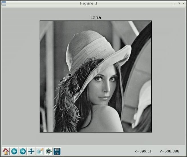
The plt.xticks([]) and plt.yticks([]) functions can be used to disable x and y axis. Run the preceding code again, and this time, comment out the two lines with the plt.xticks([]) and plt.yticks([]) functions.
The cv2.imread() OpenCV function reads images and saves them as NumPy arrays of Blue, Green, and Red (BGR) pixels.
However, plt.imshow() displays images in the RGB format. So, if we read an image as it is with cv2.imread() and display it using plt.imshow(), then the value for blue will be treated as the value for red and vice versa by plt.imshow(), and it will display an image with distorted colors. Try out the preceding code with the following alterations in the respective lines to experience the concept:
img = cv2.imread('lena_color_512.tif',1)
plt.imshow(img)
To remedy this issue, we need to convert an image read in the BGR format into an RGB array format by cv2.imread()so that plt.imshow() will be able to render it in a way that makes sense to us. We will be using the cv2.cvtColor() function for this, which we will learn soon.
Note
Explore this URL to get more information on matplotlib: http://matplotlib.org/.
Using matplotlib
We can also use matplotlib to display images. matplotlib is a 2D plotting library for Python. It provides a wide range of plotting options, which we will be using in the next chapter. Let's look at a basic example of matplotlib:
import cv2
import matplotlib.pyplot as plt
#Program to load a color image in gray scale and to display using matplotlib
img = cv2.imread('lena_color_512.tif',0)
plt.imshow(img,cmap='gray')
plt.title('Lena')
plt.xticks([])
plt.yticks([])
plt.show()
In this example, we are reading an image in grayscale and displaying it using matplotlib. The following screenshot shows the plot of the image:

The plt.xticks([]) and plt.yticks([]) functions can be used to disable x and y axis. Run the preceding code again, and this time, comment out the two lines with the plt.xticks([]) and plt.yticks([]) functions.
The cv2.imread() OpenCV function reads images and saves them as NumPy arrays of Blue, Green, and Red (BGR) pixels.
However, plt.imshow() displays images in the RGB format. So, if we read an image as it is with cv2.imread() and display it using plt.imshow(), then the value for blue will be treated as the value for red and vice versa by plt.imshow(), and it will display an image with distorted colors. Try out the preceding code with the following alterations in the respective lines to experience the concept:
img = cv2.imread('lena_color_512.tif',1)
plt.imshow(img)
To remedy this issue, we need to convert an image read in the BGR format into an RGB array format by cv2.imread()so that plt.imshow() will be able to render it in a way that makes sense to us. We will be using the cv2.cvtColor() function for this, which we will learn soon.
Note
Explore this URL to get more information on matplotlib: http://matplotlib.org/.
Working with Webcam using OpenCV
OpenCV has a functionality to work with standard USB webcams. Let's take a look at an example to capture an image from a webcam:
import cv2

# initialize the camera
cam = cv2.VideoCapture(0)
ret, image = cam.read()

if ret:
    cv2.imshow('SnapshotTest',image)
    cv2.waitKey(0)
    cv2.destroyWindow('SnapshotTest')
    cv2.imwrite('/home/pi/book/output/SnapshotTest.jpg',image)
cam.release()
In the preceding code, cv2.VideoCapture() creates a video capture object. The argument for it can either be a video device or a file. In this case, we are passing a device index, which is 0. If we have more cameras, then we can pass the appropriate device index based on what camera to choose. If you have one camera, just pass 0.
You can find out the number of cameras and associated device indexes using the following command:
ls -l /dev/video*
Once cam.read() returns a Boolean value ret and the frame which is the image it captured. If the image capture is successful, then ret will be True; otherwise, it will be False. The previously listed code will capture an image with the camera device, /dev/video0, display it, and then save it. cam.release() will release the device.
This code can be used with slight modifications to display live video stream from the webcam:
import cv2

cam = cv2.VideoCapture(0)
print 'Default Resolution is ' + str(int(cam.get(3))) + 'x' + str(int(cam.get(4)))
w=1024
h=768
cam.set(3,w)
cam.set(4,h)
print 'Now resolution is set to ' + str(w) + 'x' + str(h)

while(True):
    # Capture frame-by-frame
    ret, frame = cam.read()

    # Display the resulting frame
    cv2.imshow('Video Test',frame)

    # Wait for Escape Key
    if cv2.waitKey(1) == 27 :
        break

# When everything done, release the capture
cam.release()
cv2.destroyAllWindows()
You can access the features of the video device with cam.get(propertyID). 3 stands for the width and 4 stands for the height. These properties can be set with cam.set(propertyID, value).
The preceding code first displays the default resolution and then sets it to 1024 x 768 and displays the live video stream till the Esc key is pressed. This is the basic skeleton logic for all the live video processing with OpenCV. We will make use of this in future.
Saving a video using OpenCV
We need to use the cv2.VideoWriter() function to write a video to a file. Take a look at the following code:
import cv2
cam = cv2.VideoCapture(0)
output = cv2.VideoWriter('VideoStream.avi',
cv2.cv.CV_FOURCC(*'WMV2'),40.0,(640,480))

while (cam.isOpened()):
    ret, frame = cam.read()
    if ret == True:
        output.write(frame)
        cv2.imshow('VideoStream', frame )
        if cv2.waitKey(1) == 27 :
            break
    else:
        break

cam.release()
output.release()
cv2.destroyAllWindows()
In the preceding code, cv2.VideoWriter() accepts the following parameters:
- Filename: This is the name of the video file.
- FourCC: This stands for Four Character Code. We have to use the
cv2.cv.CV_FOURCC()function for this. This function accepts FourCC in the *'code' format. This means that for DIVX, we need to pass *'DIVX', and so on. Some supported formats are DIVX, XVID, H264, MJPG, WMV1, and WMV2.Note
You can read more about FourCC at www.fourcc.org.
- Framerate: This is the rate of the frames to be captured per second.
- Resolution: This is the resolution of the video to be captured.
The preceding code records the video till the Esc key is pressed and saves it in the specified file.
Pi Camera and OpenCV
The following code demonstrates the use of Picamera with OpenCV. It shows a preview for 3 seconds, captures an image, and displays it on screen using cv2.imshow():
import picamera
import picamera.array
import time
import cv2

with picamera.PiCamera() as camera:
    rawCap=picamera.array.PiRGBArray(camera)
    camera.start_preview()
    time.sleep(3)
    camera.capture(rawCap,format="bgr")
    image=rawCap.array
cv2.imshow("Test",image)
cv2.waitKey(0)
cv2.destroyAllWindows()
Saving a video using OpenCV
We need to use the cv2.VideoWriter() function to write a video to a file. Take a look at the following code:
import cv2
cam = cv2.VideoCapture(0)
output = cv2.VideoWriter('VideoStream.avi',
cv2.cv.CV_FOURCC(*'WMV2'),40.0,(640,480))

while (cam.isOpened()):
    ret, frame = cam.read()
    if ret == True:
        output.write(frame)
        cv2.imshow('VideoStream', frame )
        if cv2.waitKey(1) == 27 :
            break
    else:
        break

cam.release()
output.release()
cv2.destroyAllWindows()
In the preceding code, cv2.VideoWriter() accepts the following parameters:
- Filename: This is the name of the video file.
- FourCC: This stands for Four Character Code. We have to use the
cv2.cv.CV_FOURCC()function for this. This function accepts FourCC in the *'code' format. This means that for DIVX, we need to pass *'DIVX', and so on. Some supported formats are DIVX, XVID, H264, MJPG, WMV1, and WMV2.Note
You can read more about FourCC at www.fourcc.org.
- Framerate: This is the rate of the frames to be captured per second.
- Resolution: This is the resolution of the video to be captured.
The preceding code records the video till the Esc key is pressed and saves it in the specified file.
Pi Camera and OpenCV
The following code demonstrates the use of Picamera with OpenCV. It shows a preview for 3 seconds, captures an image, and displays it on screen using cv2.imshow():
import picamera
import picamera.array
import time
import cv2

with picamera.PiCamera() as camera:
    rawCap=picamera.array.PiRGBArray(camera)
    camera.start_preview()
    time.sleep(3)
    camera.capture(rawCap,format="bgr")
    image=rawCap.array
cv2.imshow("Test",image)
cv2.waitKey(0)
cv2.destroyAllWindows()
Pi Camera and OpenCV
The following code demonstrates the use of Picamera with OpenCV. It shows a preview for 3 seconds, captures an image, and displays it on screen using cv2.imshow():
import picamera
import picamera.array
import time
import cv2

with picamera.PiCamera() as camera:
    rawCap=picamera.array.PiRGBArray(camera)
    camera.start_preview()
    time.sleep(3)
    camera.capture(rawCap,format="bgr")
    image=rawCap.array
cv2.imshow("Test",image)
cv2.waitKey(0)
cv2.destroyAllWindows()
Retrieving image properties
We can retrieve and use many image properties with OpenCV functions. Take a look at the following code:
import cv2
img = cv2.imread('lena_color_512.tif',1)
print img.shape
print img.size
print img.dtype
The img.shape operation returns the shape of the image, that is, its dimensions and the number of color channels. The output of the previously listed code will be as follows:
(512, 512, 3)
786432
uint8
If the image is colored, then img.shape returns a triplet containing the number of rows, the number of columns, and the number of channels in the image. Usually, the number of channels is three, representing the red, green, and blue channels. If the image is grayscale, then img.shape only returns the number of rows and the number of columns. Try to modify the preceding code to read the image in the grayscale mode and observe the output of img.shape.
The img.size operation returns the total number of pixels, and img.dtype returns the image datatype.
Arithmetic operations on images
In this section, we will take a look at the various arithmetic operations that can be performed on images. Images are represented as matrices in OpenCV. So, arithmetic operations on images are the same as arithmetic operations on matrices. Images must be of the same size in order to perform arithmetic operations with images, and these operations are performed on individual pixels .cv2.add() method is used to add two images, where images are passed as parameters.
The cv2.subtract() method is used to subtract one image from another.
Note
We know that subtraction operation is not commutative; so, cv2.subtract(img1,img2) and cv2.(img2,img1) will yield different results, whereas cv2.add(img1,img2) and cv2.add(img2,img1) will yield the same result as the addition operation is commutative. Both the images have to be of the same size and type as that explained earlier.
Check out the following code:
import cv2
img1 = cv2.imread('4.2.03.tiff',1)
img2 = cv2.imread('4.2.04.tiff',1)
cv2.imshow('Image1',img1)
cv2.waitKey(0)
cv2.imshow('Image2',img2)
cv2.waitKey(0)
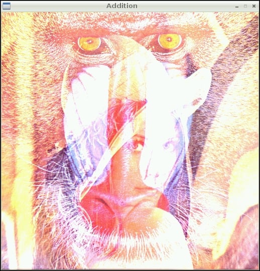
cv2.imshow('Addition',cv2.add(img1,img2))
cv2.waitKey(0)
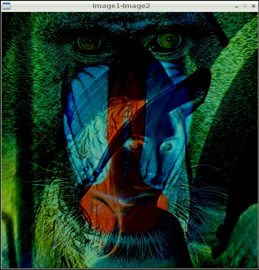
cv2.imshow('Image1-Image2',cv2.subtract(img1,img2))
cv2.waitKey(0)
cv2.imshow('Image2-Image1',cv2.subtract(img2,img1))
cv2.waitKey(0)
cv2.destroyAllWindows()
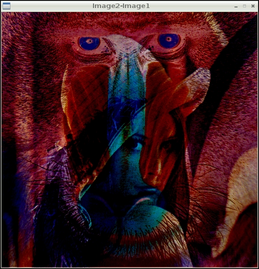
The preceding code demonstrates the usage of arithmetic functions on images. Image2 is the same Lena image that we experimented with in the previous chapter, so I am not including its output window. The following is the output window of Image1:

The following is the output of the Addition:
The following is the output window of Image1-Image2:
The following is the output window if Image2-Image1:
Splitting and merging image color channels
On several occasions, we might be interested in working separately with the red, green, and blue channels. For example, we might want to build a histogram for each channel of an image.
The cv2.split() method is used to split an image into three different intensity arrays for each color channel, whereas cv2.merge() is used to merge different arrays into a single multichannel array, that is, a color image. Let's take a look at an example:
import cv2
img = cv2.imread('4.2.03.tiff',1)
b,g,r = cv2.split (img)
cv2.imshow('Blue Channel',b)
cv2.imshow('Green Channel',g)
cv2.imshow('Red Channel',r)
img=cv2.merge((b,g,r))
cv2.imshow('Merged Output',img)
cv2.waitKey(0)
cv2.destroyAllWindows()
The preceding program first splits the image into three channels (blue, green, and red) and then displays each one of them. The separate channels will only hold the intensity values of that color, and they will be essentially displayed as grayscale intensity images. Then, the program will merge all the channels back into an image and display it.
Negating an image
In mathematical terms, the negative of an image is the inversion of colors. For a grayscale image, it is even simpler! The negative of a grayscale image is just the intensity inversion, which can be achieved by finding the complement of the intensity from 255. A pixel value ranges from 0 to 255 and, therefore, negation is the subtraction of the pixel value from the maximum value, that is, 255. The code for this is as follows:
import cv2
img = cv2.imread('4.2.07.tiff')
grayscale = cv2.cvtColor(img,cv2.COLOR_BGR2GRAY)
negative = abs(255-grayscale)
cv2.imshow('Original',img)
cv2.imshow('Grayscale',grayscale)
cv2.imshow('Negative',negative)
cv2.waitKey(0)
cv2.destroyAllWindows()
Tip
The negative of a negative will be the original grayscale image. Try this on your own by taking the image negative of a negative again.
Logical operations on images
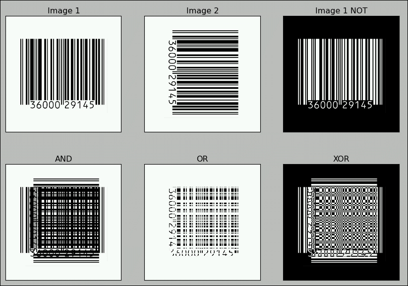
OpenCV provides bitwise logical operation functions on images. We will take a look at functions that provide bitwise logical AND, OR, XOR (exclusive OR), and NOT (inversion) functionalities. These functions can be better demonstrated visually with grayscale images. I am going to use barcode images in horizontal and vertical orientations for demonstration. Look at the following code:
import cv2
import matplotlib.pyplot as plt

img1 = cv2.imread('Barcode_Hor.png',0)
img2 = cv2.imread('Barcode_Ver.png',0)
not_out=cv2.bitwise_not(img1)
and_out=cv2.bitwise_and(img1,img2)
or_out=cv2.bitwise_or(img1,img2)
xor_out=cv2.bitwise_xor(img1,img2)

titles = ['Image 1','Image 2','Image 1 NOT','AND','OR','XOR']
images = [img1,img2,not_out,and_out,or_out,xor_out]

for i in xrange(6):
    plt.subplot(2,3,i+1)
    plt.imshow(images[i],cmap='gray')
    plt.title(titles[i])
    plt.xticks([]),plt.yticks([])
plt.show()
We first read images in the grayscale mode and calculate the NOT, AND, OR, and XOR, and then, with matplotlib, we display them in a neat way. We are leveraging the plt.subplot() function here to display multiple images. In this example, we are creating a two row and three column grid for our images and displaying each image in every part of the grid. You can modify this line and make it plt.subplot(3,2,i+1) in order to create a three row and two column grid.
We can do this without a loop in the following way. For each image, you have to write the following statements. I am writing this for the first image here only. Go ahead and write it for the rest of the five images:
plt.subplot(2,3,1) , plt.imshow(img1,cmap='gray') , plt.title('Image 1') , plt.xticks([]),plt.yticks([])Finally, use plt.show() to display. This technique is to avoid the loop where there is very small number of images to be displayed: usually 2 or 3. The output of this will be exactly the same, as follows:
Note
You might want to make a note of the fact that a logical NOT operation is the negative of the image.
You can check out the Python OpenCV API documentation at http://docs.opencv.org/modules/refman.html.
Colorspaces and conversions
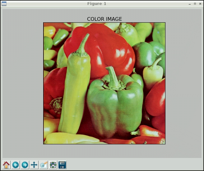
A colorspace is a mathematical model used to represent colors. Usually, colorspaces are used to represent colors in a numerical form and perform mathematical and logical operations with them. In this book, the colorspaces we mostly use are BGR (OpenCV's default colorspace), RGB, HSV, and grayscale. BGR stand for Blue, Green, and Red. HSV represents colors in the Hue, Saturation, and Value format. OpenCV has a cv2.cvtColor(img,conv_flag) function that allows us to change the colorspace of an img image, while the source and target colorspaces are indicated in the conv_flag parameter. We have learned that OpenCV loads images in the BGR format, and matplotlib uses the RGB format for images. So, before displaying images with matplotlib, we need to convert images from BGR to the RGB colorspace. Take a look at the following code. The programs read image in the color mode using cv2.imread(), which imports the image in the BGR colorspace. Then, it converts it into RGB using cv2.cvtColor(), and finally, it uses matplotlib to display the image:
import cv2
import matplotlib.pyplot as plt

img = cv2.imread('4.2.07.tiff',1)
img = cv2.cvtColor( img , cv2.COLOR_BGR2RGB )
plt.imshow( img ), plt.title('COLOR IMAGE'), plt.xticks([]), plt.yticks([])
plt.show()
Another way to convert an image from BGR to RGB is to first split the image into three separate channels (B, G, and R channels) and merge them in the BGR order. However, this takes more time as split and merge operations are inherently computationally costly, making them slower and inefficient. The following code shows this method:
import cv2
import matplotlib.pyplot as plt
img = cv2.imread('4.2.07.tiff',1)
b,g,r = cv2.split( img )
img=cv2.merge((r,g,b))
plt.imshow( img ), plt.title('COLOR IMAGE'), plt.xticks([]), plt.yticks([])
plt.show()
The output of both the programs is the same as that shown in the following screenshot:
If you need to know the colorspace conversion flags, then the following snippet of code will assist you in finding the list of available flags for your current OpenCV installation:
import cv2
j=0
for filename in dir(cv2):
    if filename.startswith('COLOR_'):
        print filename
        j=j+1

print 'There are ' + str(j) + ' Colorspace Conversion flags in OpenCV'
The last few lines of the output will be as follows (I am not including the complete output due to space limitation):
.
.
.
COLOR_YUV420P2BGRA
COLOR_YUV420P2GRAY
COLOR_YUV420P2RGB
COLOR_YUV420P2RGBA
COLOR_YUV420SP2BGR
COLOR_YUV420SP2BGRA
COLOR_YUV420SP2GRAY
COLOR_YUV420SP2RGB
COLOR_YUV420SP2RGBA
There are 176 Colorspace Conversion flags in OpenCV
The following code converts a color from BGR to HSV and prints it:
>>> import cv2
>>> import numpy as np
>>> c =  cv2.cvtColor(np.uint8[[[255,0,0]]]),cv2.COLOR_BGR2HSV)
>>> print c
[[[120 255 255]]]
The preceding snippet of code prints an HSV value of Blue represented in BGR.
Hue, Saturation, Value (HSV) is a color model that describes colors (hue or tint) in terms of their shade (the saturation or the amount of gray) and their brightness (the value or luminance). Hue is expressed as a number representing hues of red, yellow, green, cyan , blue, and magenta. Saturation is the amount of gray in the color. Value works in conjunction with saturation and describes the brightness or intensity of the color.
Tracking in real time based on color
Let's study a real-life application of this concept. In the HSV format, it's much easier to recognize the color range. If we need to track a specific color object, we will need to define a color range in HSV and then convert the captured image in the HSV format and check whether the part of that image falls within the HSV color range of our interest. We can use the cv2.inRange() function to achieve this. This function takes an image, the upper and lower bounds of the colors, and then it checks the range criteria for each pixel. If the pixel value falls in the given color range, then the corresponding pixel in the output image is 0; otherwise, it is 255, thus creating a binary mask. We can use bitwise_and() to extract the color range we're interested in using this binary mask thereafter. Take a look at the following code to understand this concept:
import numpy as np
import cv2

cam = cv2.VideoCapture(0)

while (True):
    ret, frame = cam.read()

hsv = cv2.cvtColor(frame, cv2.COLOR_BGR2HSV)

image_mask = cv2.inRange(hsv, np.array([40, 50, 50]), np.array([80, 255, 255]))

output = cv2.bitwise_and(frame, frame, mask = image_mask)

cv2.imshow('Original', frame)
cv2.imshow('Output', output)

if cv2.waitKey(1) == 27:
    break

cv2.destroyAllWindows()
cam.release()
We're tracking the green-colored objects in this program. The output should be similar to the following figure. I used green tea bag tags as the test object.
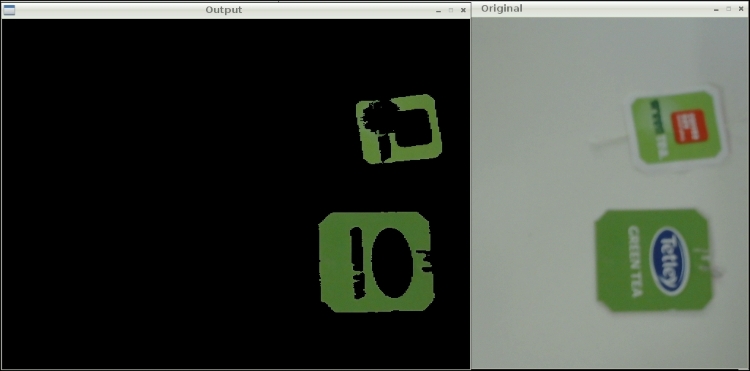
The mask image is not included in the preceding figure. You can see it yourself by adding cv2.imshow('Image Mask',image_mask) to the code. It will be a binary (pure black and white) image.
We can also track multiple colors by tweaking this code a bit. We need to modify the preceding code by creating a mask for another color range. Then, we can use cv2.add() to get the combined mask for two distinct color ranges, as follows:
blue=cv2.inRange(hsv, np.array([100,50,50]), np.array([140,255,255]))
green=cv2.inRange(hsv,np.array([40,50,50]),np.array([80,255,255]))
image_mask=cv2.add(blue,green)
output=cv2.bitwise_and(frame,frame,mask=image_mask)
Try this code and check the output by yourself.
Summary
In this chapter, we learned the basics of computer vision with OpenCV and Pi. We also went through the basic image processing operations and implemented a real-life project to track objects in a live video stream based on the color.
In the next chapter, we will learn some more advanced concepts in computer vision and implement a fully fledged motion detection system with Pi and a webcam with the use of these concepts.


