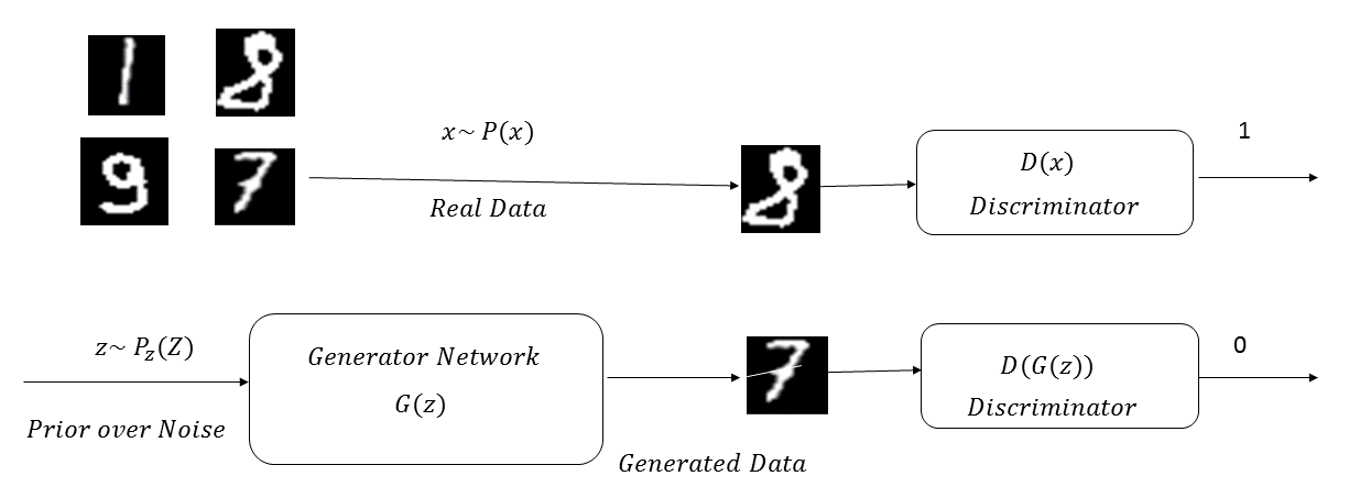
Generative adversarial networks, popularly known as GANs, are generative models that learn a specific probability distribution through a generator, G. The generator G plays a zero sum minimax game with a discriminator D and both evolve over time, before the Nash equilibrium is reached. The generator tries to produce samples similar to the ones generated by a given probability distribution, P(x), while the discriminator D tries to distinguish those fake data samples generated by the generator G from the data sample from the original distribution. The generator G tries to generate samples similar to the ones from P(x), by converting samples, z, drawn from a noise distribution, P(z). The discriminator, D, learns to tag samples generated by the generator G as G(z) when fake; x belongs to P(x) when they are original. At the equilibrium of the minimax game, the generator will learn to produce samples similar to the ones generated by the original distribution, P(x), so that the following is true:

The following diagram illustrates a GAN network learning the probability distribution of the MNIST digits:

The cost function minimized by the discriminator is the binary cross-entropy for distinguishing the real data points belonging to the probability distribution P(x) from the fake ones generated by the generator (that is, G(z)):

The generator will try to maximize the same cost function given by (1). This means that, the optimization problem can be formulated as a minimax player with the utility function U(G,D), as illustrated here:

Generally, to measure how far a given probability distribution matches that of a given distribution, f-divergence measures are used, such as the Kullback–Leibler (KL) divergence, the Jensen Shannon divergence, and the Bhattacharyya distance. For example, the KL divergence between two probability distributions, P and Q, is given by the following, where the expectation is with respect to the distribution, P:

Similarly, the Jensen Shannon divergence between P and Q is given as follows:

Now, coming back to (2), the expression can be written as follows:

Here, G(x) is the probability distribution for the generator. Expanding the expectation into its integral form, we get the following:

For a fixed generator distribution, G(x), the utility function will be at a minimum with respect to the discriminator if the following is true:

Substituting D(x) from (5) in (3), we get the following:

Now, the task of the generator is to maximize the utility,  , or minimize the utility,
  . The expression for
  can be rearranged as follows:


Hence, we can see that the generator minimizing  is equivalent to minimizing the Jensen Shannon divergence between the real distribution, P(x), and the distribution of the samples generated by the generator, G (that is, G(x)).
Training a GAN is not a straightforward process, and there are several technical considerations that we need to take into account while training such a network. We will be using an advanced GAN network to build a cross-domain style transfer application in Chapter 4, Style Transfer in Fashion Industry using GANs.


