Search icon CANCEL
Subscription
0
Cart icon
Your Cart (0 item)
Close icon
You have no products in your basket yet
Save more on your purchases! discount-offer-chevron-icon
Savings automatically calculated. No voucher code required.
Arrow left icon
Explore Products
Best Sellers
New Releases
Books
Videos
Audiobooks
Learning Hub
Free Learning
Arrow right icon
Arrow up icon
GO TO TOP
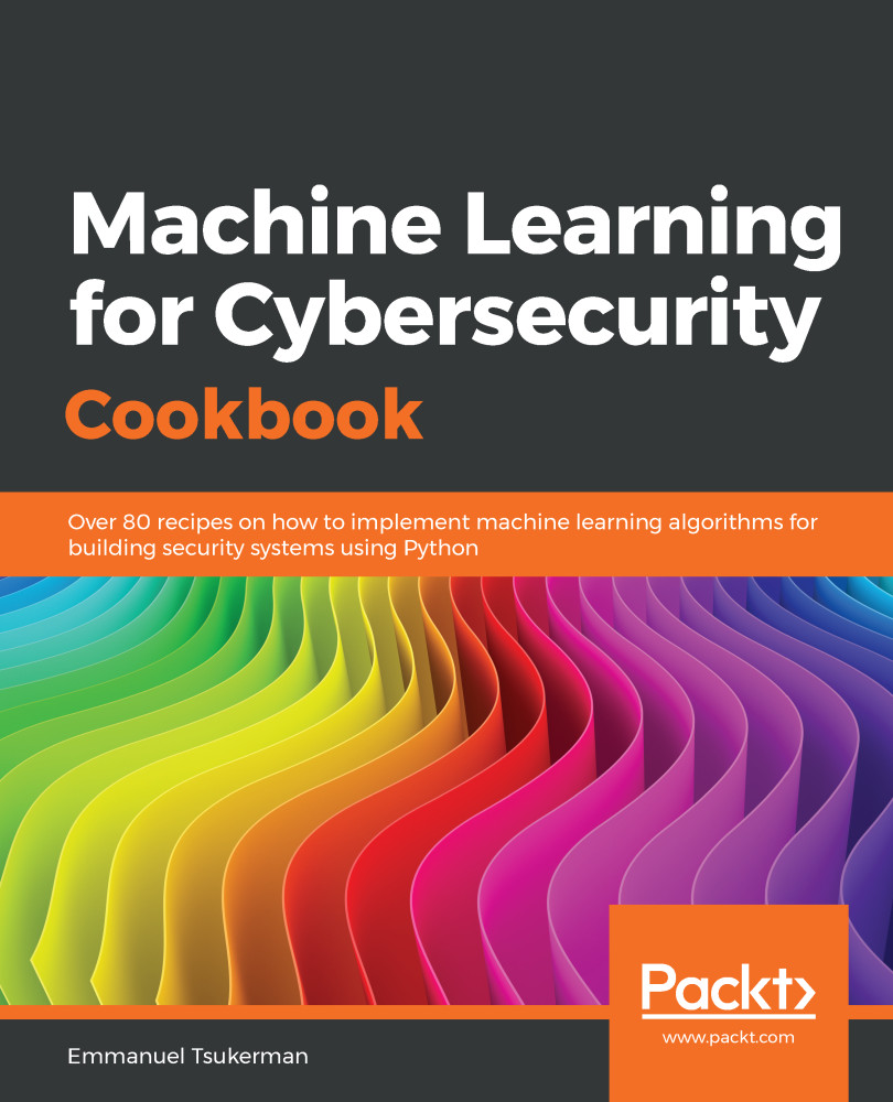
Machine Learning for Cybersecurity Cookbook

You're reading from   Machine Learning for Cybersecurity Cookbook Over 80 recipes on how to implement machine learning algorithms for building security systems using Python

Arrow left icon
Product type Paperback
Published in Nov 2019
Publisher Packt
ISBN-13 9781789614671
Length 346 pages
Edition 1st Edition
Languages
Arrow right icon
Author (1):
Arrow left icon
Emmanuel Tsukerman Emmanuel Tsukerman
Author Profile Icon Emmanuel Tsukerman
Emmanuel Tsukerman
Arrow right icon
View More author details
Toc

Table of Contents (11) Chapters Close

Preface 1. Machine Learning for Cybersecurity 2. Machine Learning-Based Malware Detection FREE CHAPTER 3. Advanced Malware Detection 4. Machine Learning for Social Engineering 5. Penetration Testing Using Machine Learning 6. Automatic Intrusion Detection 7. Securing and Attacking Data with Machine Learning 8. Secure and Private AI 9. Other Books You May Enjoy Appendix

Summarizing large data using principal component analysis

Suppose that you would like to build a predictor for an individual's expected net fiscal worth at age 45. There are a huge number of variables to be considered: IQ, current fiscal worth, marriage status, height, geographical location, health, education, career state, age, and many others you might come up with, such as number of LinkedIn connections or SAT scores.

The trouble with having so many features is several-fold. First, the amount of data, which will incur high storage costs and computational time for your algorithm. Second, with a large feature space, it is critical to have a large amount of data for the model to be accurate. That's to say, it becomes harder to distinguish the signal from the noise. For these reasons, when dealing with high-dimensional data such as this, we often employ dimensionality reduction techniques, such as PCA. More information on the topic can be found at https://en.wikipedia.org/wiki/Principal_component_analysis.

PCA allows us to take our features and return a smaller number of new features, formed from our original ones, with maximal explanatory power. In addition, since the new features are linear combinations of the old features, this allows us to anonymize our data, which is very handy when working with financial information, for example.

Getting ready

The preparation for this recipe consists of installing the scikit-learn and pandas packages in pip. The command for this is as follows:

pip install sklearn pandas

In addition, we will be utilizing the same dataset, malware_pe_headers.csv, as in the previous recipe.

How to do it...

In this section, we'll walk through a recipe showing how to use PCA on data:

  1. Start by importing the necessary libraries and reading in the dataset:
from sklearn.decomposition import PCA
import pandas as pd

data = pd.read_csv("file_pe_headers.csv", sep=",")
X = data.drop(["Name", "Malware"], axis=1).to_numpy()
  1. Standardize the dataset, as is necessary before applying PCA:
from sklearn.preprocessing import StandardScaler

X_standardized = StandardScaler().fit_transform(X)
  1. Instantiate a PCA instance and use it to reduce the dimensionality of our data:
pca = PCA()
pca.fit_transform(X_standardized)
  1. Assess the effectiveness of your dimensionality reduction:
print(pca.explained_variance_ratio_)

The following screenshot shows the output:

How it works...

We begin by reading in our dataset and then standardizing it, as in the recipe on standardizing data (steps 1 and 2). (It is necessary to work with standardized data before applying PCA). We now instantiate a new PCA transformer instance, and use it to both learn the transformation (fit) and also apply the transform to the dataset, using fit_transform (step 3). In step 4, we analyze our transformation. In particular, note that the elements of pca.explained_variance_ratio_ indicate how much of the variance is accounted for in each direction. The sum is 1, indicating that all the variance is accounted for if we consider the full space in which the data lives. However, just by taking the first few directions, we can account for a large portion of the variance, while limiting our dimensionality. In our example, the first 40 directions account for 90% of the variance:

sum(pca.explained_variance_ratio_[0:40])

This produces the following output:

0.9068522354673663

This means that we can reduce our number of features to 40 (from 78) while preserving 90% of the variance. The implications of this are that many of the features of the PE header are closely correlated, which is understandable, as they are not designed to be independent.

lock icon The rest of the chapter is locked
Register for a free Packt account to unlock a world of extra content!
A free Packt account unlocks extra newsletters, articles, discounted offers, and much more. Start advancing your knowledge today.
Unlock this book and the full library FREE for 7 days
Get unlimited access to 7000+ expert-authored eBooks and videos courses covering every tech area you can think of
Renews at $19.99/month. Cancel anytime
Banner background image