Search icon CANCEL
Subscription
0
Cart icon
Your Cart (0 item)
Close icon
You have no products in your basket yet
Save more on your purchases! discount-offer-chevron-icon
Savings automatically calculated. No voucher code required.
Arrow left icon
Explore Products
Best Sellers
New Releases
Books
Videos
Audiobooks
Learning Hub
Free Learning
Arrow right icon
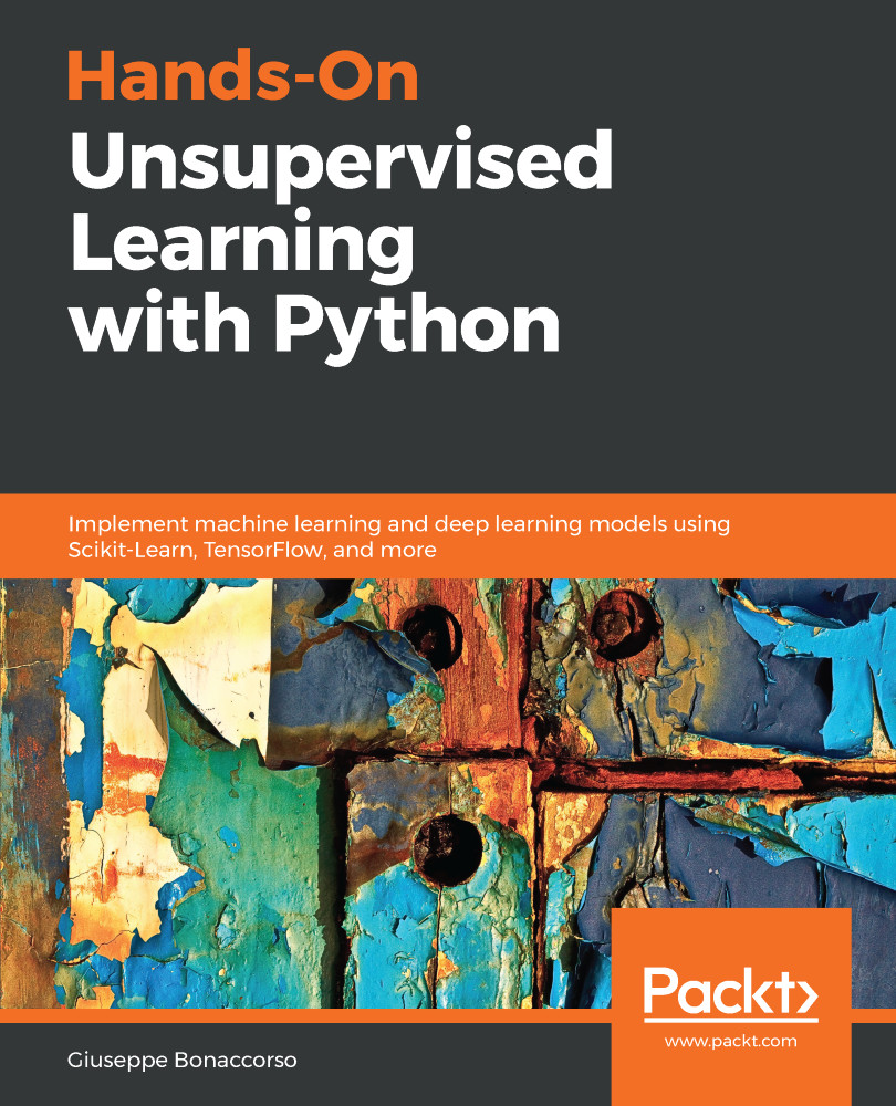
Hands-On Unsupervised Learning with Python

Hands-On Unsupervised Learning with Python: Implement machine learning and deep learning models using Scikit-Learn, TensorFlow, and more

Arrow left icon
Profile Icon Bonaccorso Profile Icon Giuseppe Bonaccorso
Arrow right icon
€8.99 €31.99
Full star icon Full star icon Full star icon Half star icon Empty star icon 3.7 (3 Ratings)
eBook Feb 2019 386 pages 1st Edition
eBook
€8.99 €31.99
Paperback
€38.99
Subscription
Free Trial
Renews at €18.99p/m
eBook
€8.99 €31.99
Paperback
€38.99
Subscription
Free Trial
Renews at €18.99p/m

What do you get with eBook?

Product feature icon Instant access to your Digital eBook purchase
Product feature icon Download this book in EPUB and PDF formats
Product feature icon Access this title in our online reader with advanced features
Product feature icon DRM FREE - Read whenever, wherever and however you want
Product feature icon AI Assistant (beta) to help accelerate your learning
OR
Modal Close icon
Payment Processing...
tick Completed

Billing Address

Table of content icon View table of contents Preview book icon Preview Book

Hands-On Unsupervised Learning with Python

Getting Started with Unsupervised Learning

In this chapter, we are going to introduce fundamental machine learning concepts, assuming that you have some basic knowledge of statistical learning and probability theory. You'll learn about the uses of machine learning techniques and the logical process that improves our knowledge about both nature and the properties of a dataset. The purpose of the entire process is to build descriptive and predictive models the can support business decisions.

Unsupervised learning aims to provide tools for data exploration, mining, and generation. In this book, you'll explore different scenarios with concrete examples and analyses, and you'll learn how to apply fundamental and more complex algorithms to solve specific problems.

In this introductory chapter, we are going to discuss:

  • Why do we need machine learning?
  • Descriptive, diagnostic, predictive, and prescriptive analyses
  • Types of machine learning
  • Why are we using Python?

Technical requirements

Why do we need machine learning?

Data is everywhere. At this very moment, thousands of systems are collecting records that make up the history of specific services, together with logs, user interactions, and many other context-dependent elements. Only a decade ago, most companies couldn't even manage 1% of their data efficiently. For this reason, databases were periodically pruned and only important data used to be retained in permanent storage servers.

Conversely, nowadays almost every company can exploit cloud infrastructures that scale in order to cope with the increasing volume of incoming data. Tools such as Apache Hadoop or Apache Spark allow both data scientists and engineers to implement complex pipelines involving extremely large volumes of data. At this point, all the barriers have been torn down and a democratized process is in place. However, what is the actual value of these large datasets? From a business viewpoint, the information is valuable only when it can help make the right decisions, reducing uncertainty and providing better contextual insight. This means that, without the right tools and knowledge, a bunch of data is only a cost to the company that needs to be limited to increase the margins.

Machine learning is a large branch of computer science (in particular, artificial intelligence), which aims to implement descriptive and predictive models of reality by exploiting existing datasets. As this book is dedicated to practical unsupervised solutions, we are going to focus only on algorithms that describe the context by looking for hidden causes and relationships. However, even if only from a theoretical viewpoint, it's helpful to show the main differences between machine learning problems. Only complete awareness (not limited to mere technical aspects) of the goals can lead to a rational answer to the initial question, Why do we need machine learning?

We can start by saying that human beings have extraordinary cognitive abilities, which have inspired many systems, but they lack analytical skills when the number of elements increases significantly. For example, if you're a teacher who is meeting his/her class for the first time, you'll be able to compute a rough estimate of the percentage of female students after taking a glance at the entire group. Usually, the estimate is likely to be accurate and close to the actual count, even if the estimation is made by two or more individuals. However, if we repeat the experiment with the entire population of a school gathered in a courtyard, the distinction of gender will not be evident. This is because all students are clearly visible in the class; however, telling the sexes apart in the courtyard is limited by certain factors (for example, taller people can hide shorter ones). Getting rid of the analogy, we can say that a large amount of data usually carries a lot of information. In order to extract and categorize the information, it's necessary to take an automated approach.

Before moving to the next section, let's discuss the concepts of descriptive, diagnostic, predictive, and prescriptive analyses, originally defined by Gartner. However, in this case, we want to focus on a system (for example, a generic context) that we are analyzing in order to gain more and more control over its behavior.

The complete process is represented in the following diagram:

Descriptive, diagnostic, predictive, and prescriptive flow

Descriptive analysis

The first problem to solve in almost any data science scenario concerns understanding its nature. We need to know how the system works or what a dataset is describing. Without this analysis, our knowledge is too limited to make any assumption or hypothesis. For example, we can observe a chart of the average temperature in a city for several years. If we are unable to describe the time series discovering the correlation, seasonalities, and trends, any other question remains unsolved. In our specific context, if we don't discover the similarities between groups of objects, we cannot try to find out a way to summarize their common features. The data scientist has to employ specific tools for every particular problem, but, at the end of this stage, all possible (and helpful) questions must be answered.

Moreover, as this process must have clear business value, it's important to involve different stakeholders with the purpose of gathering their knowledge and converting it into a common language. For example, when working with healthcare data, a physician might talk about hereditary factors, but for our purpose, it's preferable to say that there's a correlation among some samples, so we're not fully authorized to treat them as statistically independent elements. In general, the outcome of descriptive analysis is a summary containing all metric evaluations and conclusions that are necessary to qualify the context, and reducing uncertainty. In the example of the temperature chart, the data scientist should be able to answer the auto-correlation, the periodicity of the peaks, the number of potential outliers, and the presence of trends.

Diagnostic analysis

Till now, we have worked with output data, which has been observed after a specific underlying process has generated it. The natural question after having described the system relates to the causes. Temperature depends on many meteorological and geographical factors, which can be either easily observable or completely hidden. Seasonality in the time series is clearly influenced by the period of the year, but what about the outliers?

For example, we have discovered a peak in a region identified as winter. How can we justify it? In a simplistic approach, this can be considered as a noisy outlier that can be filtered out. However, if it has been observed and there's a ground truth behind the measure (for example, all the parties agree that it's not an error), we should assume the presence of a hidden (or latent) cause.

It can be surprising, but the majority of more complex scenarios are characterized by a huge number of latent causes (sometimes called factors) that are too difficult to analyze. In general, this is not a bad condition but, as we're going to discuss, it's important to include them in the model to learn their influence through the dataset.

On the other hand, deciding to drop all unknown elements means reducing the predictive ability of the model with a proportional loss of accuracy. Therefore, the primary goal of diagnostic analysis is not necessarily to find out all the causes but to list the observable and measurable elements (known as factors), together with all the potential latent ones (which are generally summarized into a single global element).

To a certain extent, a diagnostic analysis is often similar to a reverse-engineering process, because we can easily monitor the effects, but it's more difficult to detect existing relationships between potential causes and observable effects. For this reason, such an analysis is often probabilistic and helps find the probability that a certain identified cause brings about a specific effect. In this way, it's also easier to exclude non-influencing elements and to determine relationships that were initially excluded. However, this process requires a deeper knowledge of statistical learning methods and it won't be discussed in this book, apart from a few examples, such as a Gaussian mixture.

Predictive analysis

Once the overall descriptive knowledge has been gathered and the awareness about the underlying causes is satisfactory, it's possible to create predictive models. The goal of these models is to infer future outcomes according to the history and the structure of the model itself. In many cases, this phase is analyzed together with the next one because we are seldom interested in a free evolution of the system (for example, how the temperature will change in the next month), but rather in the ways we can influence the output.

That said, let's focus only on the predictions, considering the most important elements that should be taken into account. The first consideration is about the nature of the processes. We don't need machine learning for deterministic processes unless their complexity is so high that we're forced to consider them as black boxes. The vast majority of examples we are going to discuss are about stochastic processes where the uncertainty cannot be removed. For example, we know that the temperature in a day can be modeled as a conditional probability (for example, a Gaussian) dependent on the previous observations. Therefore, a prediction sets out not to turn the system into a deterministic one, which is impossible, but to reduce the variance of the distribution, so that the probability is high only for a short range of temperatures. On the other hand, as we know that many latent factors work behind the scene, we can never accept a model based on spiky distributions (for example, on a single outcome with probability 1) because this choice would have a terribly negative impact on the final accuracy.

If our model is parameterized with variables subject to the learning process (for example, the means and covariance matrices of the Gaussians), our goal is to find out the optimal balance in the so-called bias-variance trade-off. As this chapter is an introductory one, we are not formalizing the concepts with mathematical formulas, but we need a practical definition (further details can be found in Bonaccorso G., Mastering Machine Learning Algorithms, Packt, 2018).

The common term to define a statistical predictive model is an estimator. Hence the bias of an estimator is the measurable effect of incorrect assumptions and learning procedures. In other words, if the mean of a process is 5.0 and our estimations have a mean of 3.0, we can say the model is biased. Considering the previous example, we are working with a biased estimator if the expected value of the error between the observed value and the prediction is not null. It's important to understand that we are not saying that every single estimation must have a null error, but while collecting enough samples and computing the mean, its value should be very close to zero (it can be zero only with infinite samples). Whenever it is rather larger than zero, it means that our model is not able to predict training values correctly. It's obvious that we are looking for unbiased estimators that, on average, yield accurate predictions.

On the other hand, the variance of an estimator is a measure of the robustness in the presence of samples not belonging to the training set. At the beginning of this section, we said that our processes are normally stochastic. This means that any dataset must be considered as drawn from a specific data-generating process pdata. If we have enough representative elements xi ∈ X, we can suppose that training a classifier using the limited dataset X leads to a model that is able to classify all potential samples that can be drawn from pdata.

For example, if we need to model a face classifier whose context is limited to portraits (no further face poses are allowed), we can collect a number of portraits of different individuals. Our only concern is not to exclude categories that can be present in real life. Let's assume that we have 10,000 images of individuals of different ages and genders, but we don't have any portraits with a hat. When the system is in production, we receive a call from our customer saying that the system misclassifies many pictures. After analysis, we discover that they always represent people wearing hats. It's clear that our model is not responsible for the error because it has been trained with samples representing only a region of the data generating process. Therefore, in order to solve the problem, we collect other samples and we repeat the training process. However, now we decide to use a more complex model, expecting that it will work better. Unfortunately, we observe a worse validation accuracy (for example, the accuracy on a subset that is not used in the training phase), together with a higher training accuracy. What happened here?

When an estimator learns to classify the training set perfectly but its ability on never-seen samples is poor, we say that it is overfitted and its variance is too high for the specific task (conversely, an underfitted model has a large bias and all predictions are very inaccurate). Intuitively, the model has learned too much about the training data and it has lost the ability to generalize. To better understand this concept, let's look at a Gaussian data generating process, as shown in the following graph:


Original data generating process (solid line) and sampled data histogram

If the training set hasn't been sampled in a perfectly uniform way or it's partially unbalanced (some classes have fewer samples than the other ones), or if the model is prone to overfitting, the result can be represented by an inaccurate distribution, as follows:

Learned distribution

In this case, the model has been forced to learn the details of the training set until it has excluded many potential samples from the distribution. The result is no more Gaussian, but a double-peaked distribution, where some probabilities are erroneously low. Of course, the test and validation sets are sampled from the small regions not covered by the training set (as there's no overlap between training data and validation data), therefore the model will fail in its task providing completely incorrect results.

In other words, we can say that the variance is too high because the model has learned to work with too many details, increasing the range of possibilities of different classifications over a reasonable threshold. For example, the portrait classifier could have learned that people with blue glasses are always male in the age range 30–40 (this is an unrealistic situation because the detail level is generally very low, however, it's helpful to understand the nature of the problem).

We can summarize by saying that a good predictive model must have very low bias and proportionally low variance. Unfortunately, it's generally impossible to minimize both measures effectively, so a trade-off must be accepted.

A system with a good generalization ability will be likely to have a higher bias because it is unable to capture all the details. Conversely, a high variance allows a very small bias, but the ability of the model is almost limited to the training set. In this book, we are not going to talk about classifiers, but you should perfectly understand these concepts in order to be always aware of the different behaviors that you can encounter while working on projects.

Prescriptive analysis

The primary goal of this is to answer the question How can I influence the output of the system? In order to avoid confusion, it's preferable to translate this concept into pure machine learning language, hence the question could be Which input values are necessary to obtain a specific output?

As discussed in the previous section, this phase is often merged together with predictive analysis because the models are generally employed for both tasks. However, there are specific situations where the prediction is limited to a null-input evolution (such as in the temperature example) and more complex models must be analyzed in the prescriptive stage. The main reason resides in the ability to control all the causes that are responsible for a specific output.

Sometimes, when not necessary, they are only superficially analyzed. It can happen either when the causes are not controllable (for example, meteorological events), or when it's simpler to include a global latent parameter set. The latter option is very common in machine learning and many algorithms have been developed to work efficiently with the presence of latent factors (for example, EM or SVD recommendation systems). For this reason, we are not focusing on this particular aspect, (which is extremely important in system theory) and, at the same time, we are implicitly assuming that our models provide the ability to investigate many possible outputs resulting from different inputs.

For example, in deep learning, it's possible to create inverse models that produce saliency maps of the input space, forcing a specific output class. Considering the example of the portrait classifier, we could be interested in discovering which visual elements influence the output of a class. Diagnostic analysis is generally ineffective because the causes are extremely complex and their level is too low (for example, the shape of a contour). Therefore, inverse models can help solve the prescriptive problem by showing the influence of different geometric regions. However, a complete prescriptive analysis is beyond the scope of this book and, in many cases, it's not necessary, hence we are not considering such a step in upcoming chapters. Let's now analyze the different types of machine learning algorithm.

Types of machine learning algorithm

At this point, we can briefly introduce the different types of machine learning, focusing on their main peculiarities and differences. In the following sections, we'll discuss informal definitions followed by more formal ones. If you are not familiar with the mathematical concepts involved in the discussion, you can skip the details. However, it's highly advisable to study all unknown theoretical elements, as they are fundamental to understanding the concepts analyzed in the next chapters.

Supervised learning algorithms

In a supervised scenario, the task of the model is to find the correct label of a sample, assuming that the presence of a training set is correctly labeled, along with the possibility of comparing the estimated value with the correct one. The term supervised is derived from the idea of an external teaching agent that provides precise and immediate feedback after each prediction. The model can use such feedback as a measure of the error and, consequently perform the corrections needed to reduce it.

More formally, if we assume a data generating process, the dataset is obtained as:

As discussed in the previous section, all samples must be independent and identically distributed (IID) values uniformly sampled from the data generating process. In particular, all classes must represent the actual distribution (for example, if p(y=0) = 0.4 and p(y=1) = 0.6, the proportion should 40% or 60%). However, in order to avoid biases, when the discrepancies between classes are not very large, a reasonable choice is a perfectly uniform sampling and has the same number of representatives for y=1, 2, ..., M.

A generic classifier can be modeled in two ways:

  • A parametrized function that outputs the predicted class
  • A parametrized probability distribution that outputs the class probability for every input sample

In the first case, we have:

Considering the whole dataset X, it's possible to compute a global cost function L:

As L depends only on the parameter vector (xi and yi are constants), a generic algorithm must find the optimal parameter vector that minimizes the cost function. For example, in a regression problem (where the labels are continuous), the error measure can be the squared error between the actual value and prediction:

Such a cost function can be optimized in different ways (peculiar to specific algorithms), but a very common strategy (above all in deep learning) is to employ the Stochastic Gradient Descent (SGD) algorithm. It consists of an iteration of the following two steps:

  • Computing the gradient ∇L (with respect to the parameter vector) with a small batch of samples xi ∈ X
  • Updating the weights and moving the parameters in the opposite direction of the gradient -∇L (remember that the gradient is always directed towards a maximum)

Instead, when the classifier is probabilistic, it should be represented as a parametrized conditional probability distribution:

In other words, the classifier will now output the probability of a label y given an input vector. The goal is now to find the optimal parameter set, which will obtain:

In the preceding formula, we have expressed pdata as a conditional distribution. The optimization can be obtained using a probabilistic distance metric, such as the Kullback-Leibler divergence DKL (which is always non-negative DKL 0 and DKL = 0 only when the two distributions are identical):

With a few simple manipulations, we obtain:

Therefore, the resulting cost function corresponds to the difference between the cross-entropy between p and pdata up to a constant value (the entropy of the data generating process). Therefore, the training strategy is now based on representing labels using one-hot encoding (for example, if there are two labels 0 → (0, 1) and 1 → (1, 0), so that the sum of all elements must be always equal to 1) and using an intrinsic probabilistic output (such as in a logistic regression) or a softmax filter, which transforms M values into a probability distribution.

In both cases, it's clear the presence of a hidden teacher provides a consistent measure of the error, allowing the model to correct the parameters accordingly. In particular, the second approach is extremely helpful for our purposes, therefore I recommend studying it further if it's not known well (all the main definitions can also be found in Bonaccorso G., Machine Learning Algorithms, Second Edition, Packt, 2018).

We can now discuss a very basic example of supervised learning, a linear regression model that can be employed to predict the evolution of a simple time series.

Supervised hello world!

In this example, we want to show how to perform a simple linear regression with bidimensional data. In particular, let's assume that we have a custom dataset containing 100 samples, as follows:

import numpy as np
import pandas as pd

T = np.expand_dims(np.linspace(0.0, 10.0, num=100), axis=1)
X = (T * np.random.uniform(1.0, 1.5, size=(100, 1))) + np.random.normal(0.0, 3.5, size=(100, 1))
df = pd.DataFrame(np.concatenate([T, X], axis=1), columns=['t', 'x'])
We have also created a pandas DataFrame because it's easier to create plots using the seaborn library (https://seaborn.pydata.org). In the book, the code for the plots (using Matplotlib or seaborn) is normally omitted, but it's always present in the repository.

We want to express the dataset in a synthetic way, as follows:

This task can be carried out using a linear regression algorithm, as follows:

from sklearn.linear_model import LinearRegression

lr = LinearRegression()
lr.fit(T, X)

print('x(t) = {0:.3f}t + {1:.3f}'.format(lr.coef_[0][0], lr.intercept_[0]))

The output of the last command is the following:

x(t) = 1.169t + 0.628

We can also get visual confirmation, drawing the dataset together with the regression line, as shown in the following graph:

Dataset and regression line

In this example, the regression algorithm minimized a squared error cost function, trying to reduce the discrepancy between the predicted value and the actual one. The presence of Gaussian (with null mean) noise has a minimum impact on the slope, thanks to the symmetric distribution.

Unsupervised learning algorithms

In an unsupervised scenario, as it's easy to imagine, there is no hidden teacher, hence the main goals cannot be related to minimizing the prediction error with respect to the ground truth. Indeed, the same concept of ground truth has a slightly different meaning in this context. In fact, when working with classifiers, we want to have a null error for the training samples (meaning that other classes than the true ones are never accepted as correct).

Conversely, in an unsupervised problem, we want the model to learn some pieces of information without any formal indication. This condition implies that the only elements that can be learned are the ones contained in the samples themselves. Therefore, an unsupervised algorithm is usually aimed at discovering the similarities and patterns among samples or reproducing an input distribution given a set of vectors drawn from it. Let's now analyze some of the most common categories of unsupervised models.

Cluster analysis

Cluster analysis (normally called just clustering) is an example of a task where we want to find out common features among large sets of samples. In this case, we always suppose the existence of a data generating process and we define the dataset X as:

A clustering algorithm is based on the implicit assumption that samples can be grouped according to their similarities. In particular, given two vectors, a similarity function is defined as the reciprocal or inverse of a metric function. For example, if we are working in a Euclidean space, we have:

In the previous formula, the constant ε has been introduced to avoid division by zero. It's obvious that d(a, c) < d(a, b) ⇒ s(a, c) > s(a, b). Therefore, given a representative of each cluster , we can create the set of assigned vectors considering the rule:

In other words, a cluster contains all those elements whose distance from the representative is minimum compared to all other representatives. This implies that a cluster contains samples whose similarity with the representative is maximal compared to all representatives. Moreover, after the assignment, a sample gains the right to share its feature with the other members of the same cluster.

In fact, one of the most important applications of cluster analysis is trying to increase the homogeneity of samples that are recognized as similar. For example, a recommendation engine could be based on the clustering of the user vectors (containing information about their interests and bought products). Once the groups have been defined, all the elements belonging to the same cluster are considered as similar, hence we are implicitly authorized to share the differences. If user A has bought the product P and rated it positively, we can suggest this item to user B who didn't buy it and the other way around. The process can appear arbitrary, but it turns out to be extremely effective when the number of elements is large and the feature vectors contain many discriminative elements (for example, ratings).

Generative models

Another unsupervised approach is based on generative models. The concept is not very different from what we have already discussed for supervised algorithms, but, in this case, the data generating process doesn't contain any label. Hence the goal is to model a parametrized distribution and optimize the parameters so that the distance between candidate distribution and the data generating process is minimized:

The process is generally based on the Kullback-Leibler divergence or other similar measures:

At the end of the training phase, we assume L → 0, so p ≈ pdata. In this way, we have not limited the analysis to a subset of possible samples, but rather to the entire distribution. Using a generative model allows you to draw new samples that can be very different from the ones selected for the training process, but they always belong to the same distribution. Therefore, they are (potentially) always acceptable.

For example, a Generative Adversarial Network (GAN) is a particular deep learning model that is able to learn the distribution of an image set, producing new samples that are almost indistinguishable (from a visual semantic point of view) from the training ones. As unsupervised learning is the main topic of this book, we won't dwell further on GAN in this introduction. All these concepts will be extensively discussed (with practical examples) in all the next chapters.

Association rules

The last unsupervised approach we're considering is based on the discovery of association rules and it's extremely important in the field of data mining. A common scenario is represented by a collection of commercial transactions made up of a subset of products. The goal is to find out the most important associations between products (for example, the probability of buying Pi and Pj is 70%). Specific algorithms can efficiently mine a whole database, highlighting all the relationships that can be taken into account for strategic and logistic purposes. For example, an online store can employ this method to promote all those items that are frequently bought together with other ones. Moreover, a predictive approach allows simplifying the provisioning processes by suggesting all those products that are very likely to be sold out, thanks to an increase in the sales of other items.

At this point, it's helpful to introduce the reader to a practical example of unsupervised learning. No particular prerequisites are needed, but it's preferable to have a basic knowledge of probability theory.

Unsupervised hello world!

As this book is completely dedicated to unsupervised algorithms, I've decided not to show a simple cluster analysis as a hello world! example, but rather a quite basic generative model. Let's assume that we are monitoring the number of trains that arrive at a subway station every hour because we need to ascertain the number of security agents required at the station. In particular, we're asked to have at least one agent per train and whenever there are fewer, we're going to pay a fine.

Moreover, it's easier to send a group at the beginning of every hour instead of controlling the agents one by one. As the problem is very simple, we also know that a good distribution is the Poisson one, parameterized with μ, which is also the mean. From the theory, we know that such a distribution can effectively model the random number of events happening in a fixed time frame, under the main assumption of independence. In general cases, a generative model is based on a parameterized distribution (for example, with a neural network) and no specific assumptions are made about its family. Only in some particular cases (for example, Gaussian mixture), is it reasonable to pick distributions with particular properties and, without loss of rigor, we can consider this example as one such scenario.

The probability mass function of a Poisson distribution is:

This distribution describes the probability of observing k events in a predefined interval. In our case, the interval is always one hour and we're keen to estimate the probability of observing more than 10 trains. How can we obtain the correct figure for μ?

The most common strategy is called Maximum Likelihood Estimation (MLE). It collects a set of observations and finds the value of μ that maximizes the probability that all the points have been generated by our distribution.

Assuming we have collected N observations (each observation is the number of arrivals in one hour), the likelihood of μ with respect to all samples is the joint probability of all samples (for simplicity, assumed to be IID) under the probability distribution computed using μ:

As we are working with a product and exponential, it's a common rule to compute the log-likelihood:

Once the log-likelihood has been computed, it's possible to set the derivative with respect to μ equal to 0 in order to find the optimal value. In this case, we omit the proof (which is straightforward to obtain) and arrive directly at the MLE estimation of μ:

We are lucky! The MLE estimation is just the average of the arrival times. This means that, if we have observed N values with average μ, the Poisson distribution, which is the most likely to have generated them, has μ as the characteristic coefficient. Therefore, any other sample drawn from such a distribution will be compatible with the observed dataset.

We can now start with our first simulation. Let's assume we've collected 25 observations during the early afternoon of a business day, as follows:

import numpy as np

obs = np.array([7, 11, 9, 9, 8, 11, 9, 9, 8, 7, 11, 8, 9, 9, 11, 7, 10, 9, 10, 9, 7, 8, 9, 10, 13])
mu = np.mean(obs)

print('mu = {}'.format(mu))

The output of the last command is as follows:

mu = 9.12

Hence, we have an arrival average of about nine trains per hour. The histogram is shown in the following diagram:

Histogram of the initial distribution

To compute the requested probabilities, we need to work with the Cumulative Distribution Function (CDF), which is implemented in SciPy (in the scipy.stats package). In particular, as we are interested in the probability of observing more trains than a fixed value, it's necessary to use the Survival Function (SF), which corresponds to 1-CDF, as follows:

from scipy.stats import poisson

print('P(more than 8 trains) = {}'.format(poisson.sf(8, mu)))
print('P(more than 9 trains) = {}'.format(poisson.sf(9, mu)))
print('P(more than 10 trains) = {}'.format(poisson.sf(10, mu)))
print('P(more than 11 trains) = {}'.format(poisson.sf(11, mu)))

The output of the preceding snippet is as follows:

P(more than 8 trains) = 0.5600494497386543
P(more than 9 trains) = 0.42839824517059516
P(more than 10 trains) = 0.30833234660452563
P(more than 11 trains) = 0.20878680161156604

As expected, the probability of observing more than 10 trains is low (30%) and it doesn't seem reasonable to send 10 agents. However, as our model is adaptive, we can continue collecting observations (for example, during the early morning), as follows:

new_obs = np.array([13, 14, 11, 10, 11, 13, 13, 9, 11, 14, 12, 11, 12, 14, 8, 13, 10, 14, 12, 13, 10, 9, 14, 13, 11, 14, 13, 14])

obs = np.concatenate([obs, new_obs])
mu = np.mean(obs)

print('mu = {}'.format(mu))

The new value for μ is as follows:

mu = 10.641509433962264

Now the average is almost 11 trains per hour. Assuming that we have collected enough samples (considering all potential accidents), we can re-estimate the probabilities, as follows:

print('P(more than 8 trains) = {}'.format(poisson.sf(8, mu)))
print('P(more than 9 trains) = {}'.format(poisson.sf(9, mu)))
print('P(more than 10 trains) = {}'.format(poisson.sf(10, mu)))
print('P(more than 11 trains) = {}'.format(poisson.sf(11, mu)))

The output is as follows:

P(more than 8 trains) = 0.7346243910180037
P(more than 9 trains) = 0.6193541369812121
P(more than 10 trains) = 0.49668918740243756
P(more than 11 trains) = 0.3780218948425254

With the new dataset, the probability of observing more than nine trains is about 62%, (which confirms our initial choice), but the probability of observing more than 10 trains is now about 50%. As we don't want to risk paying the fine (which is higher than the cost of an agent), it's always better to send a group of 10 agents. In order to get further confirmation, we have decided to sample 2,000 values from the distribution, as follows:

syn = poisson.rvs(mu, size=2000)

The corresponding histogram is shown in the following diagram:

Histogram of 2000 points sampled from the final Poisson distribution

The diagram confirms a peak slightly after 10 (very close to 11) and a rapid decay starting from k = 13, which has already been discovered using a limited dataset (compare the shapes of the histograms for further confirmation). However, in this case, we are generating potential samples that couldn't be present in our observation set. The MLE guarantees that the probability distribution is consistent with the data and that the new samples are weighted accordingly. This example is clearly extremely simple and its goal was only to show the dynamics of a generative model.

We are going to discuss many other more complex models and examples in the next chapters of the book. One important technique, common to many algorithms lies in not picking a predefined distribution (which implies an apriori knowledge) but rather in using flexible parametric models (for example, neural networks) to find out the optimal distribution. The choice of a predefined prior (as in this case) is justified only when there's a high confidence degree about the underlying stochastic process. In all other situations, it's always preferable to avoid any assumption and rely only on the data in order to find the most appropriate approximation of the data generating process.

Semi-supervised learning algorithms

A semi-supervised scenario can be considered as a standard supervised one that exploits some features belonging to unsupervised learning techniques. A very common problem, in fact, arises when it's easy to obtain large unlabeled datasets but the cost of labeling is very high. Hence, it's reasonable to label only a fraction of the samples and to propagate the labels to all unlabeled ones whose distance from a labeled sample is below a predefined threshold. If the dataset has been drawn from a single data generating process and the labeled samples are uniformly distributed, a semi-supervised algorithm can achieve an accuracy comparable with a supervised one. In this book, we are not discussing these algorithms; however, it's helpful to briefly introduce two very important models:

  • Label propagation
  • Semi-supervised Support Vector Machines

The first one is called label propagation and its goal is to propagate the labels of a few samples to a larger population. This goal is achieved by considering a graph where each vertex represents a sample and every edge is weighted using a distance function. Through an iterative procedure, all labeled samples will send a fraction of their label values to all their neighbors and the process is repeated until the labels stop changing. This system has a stable point (that is, a configuration that cannot evolve anymore) and the algorithm can easily reach it with a limited number of iterations.

Label propagation is extremely helpful in all those contexts where some samples can be labeled according to a similarity measure. For example, an online store could have a large base of customers, but only 10% have disclosed their gender. If the feature vectors are rich enough to represent the common behavior of male and female users, it's possible to employ the label propagation algorithm to guess the gender of customers who haven't disclosed it. Of course, it's important to remember that all the assignments are based on the assumption that similar samples have the same label. This can be true in many situations, but it can also be misleading when the complexity of the feature vectors increases.

Another important family of semi-supervised algorithms is based on the extension of standard SVM, (short for Support Vector Machine) to datasets containing unlabeled samples. In this case, we don't want to propagate existing labels, but rather the classification criterion. In other words, we want to train the classifier using the labeled dataset and extend the discriminative rule to the unlabeled samples as well.

Contrary to the standard procedure that can only evaluate unlabeled samples, a semi-supervised SVM uses them to correct the separating hyperplane. The assumption is always based on the similarity: if A has label 1 and the unlabeled sample B has d(A, B) < ε (where ε is a predefined threshold), it's reasonable to assume that the label of B is also 1. In this way, the classifier can achieve high accuracy on the whole dataset even if only a subset has been manually labeled. Similar to label propagation, these kinds of model are reliable only when the structure of the dataset is not extremely complex and, in particular, when the similarity assumption holds (unfortunately there are some cases where it's extremely difficult to find a suitable distance metric, hence many similar samples are indeed dissimilar and vice versa).

Reinforcement learning algorithms

A reinforcement learning scenario can be considered as a supervised one where the hidden teacher provides only approximate feedback after every decision of the model. More formally, reinforcement learning is characterized by continuous interaction between an agent and an environment. The former is responsible for making decisions (actions), finalized to increase its return, while the latter provides feedback to every action. Feedback is generally considered as a reward, whose value can be either positive (the action has been successful) or negative (the action shouldn't be repeated). As the agent analyzes different configurations of the environment (states), every reward must be considered as bound to the tuple (action, state). Hence, the final goal is to find a policy (a strategy that suggests the optimal action in every state) that maximizes the expected total reward.

A very classical example of reinforcement learning is an agent that learns how to play a game. During an episode, the agent tests the actions in all encountered states and collects the rewards. An algorithm corrects the policy to reduce the likelihood of non-positive actions (that is, those whose reward is positive) and increase the expected total rewards obtainable at the end of the episode.

Reinforcement learning has many interesting applications, which are not limited to games. For example, a recommendation system can correct suggestions according to binary feedback (for example, thumb up or down) provided by the user. The main difference between reinforcement and supervised learning is the information provided by the environment. In fact, in a supervised scenario, the correction is normally proportional to it, while in a reinforcement learning one it must be analyzed considering a sequence of actions and future rewards. Therefore, the corrections are normally based on the estimation of the expected reward and their effect is influenced by the value of the subsequent actions. For example, a supervised model has no memory, hence its corrections are immediate, while a reinforcement learning agent must consider the partial rollout of an episode in order to decide whether an action is actually negative or not.

Reinforcement learning is a fascinating branch of machine learning. Unfortunately, this topic is beyond the scope of this work, therefore we are not discussing it in detail (you can find further details in Hands-On Reinforcement Learning with Python, Ravichandiran S., Packt Publishing, 2018 and Mastering Machine Learning Algorithms, Bonaccorso G., Packt Publishing, 2018).

We can now briefly explain why Python has been chosen as the main language for this exploration of the world of unsupervised learning.

Why Python for data science and machine learning?

Before moving on with more technical discussions, I think it's helpful to explain the choice of Python as the programming language for this book. In the last decade, research in the field of data science and machine learning has seen exponential growth, with thousands of valuable papers and dozens of complete tools. In particular, thanks to its efficiency, elegance, and compactness, Python has been chosen by many researchers and programmers to create a complete scientific ecosystem that has been released for free.

Nowadays, packages such as scikit-learn, SciPy, NumPy, Matplotlib, pandas, and many others represent the backbone of hundreds of production-ready systems and their usage keeps growing. Moreover, complex deep learning applications such as Theano, TensorFlow, and PyTorch allow every Python user to create and train complex models without any speed limits. In fact, it's important to note that Python is not a scripting language anymore. It supports dozens of specific tasks (for example, web frameworks and graphics) and it can be interfaced with native code written in C or C++.

For such reasons, Python is an optimal choice in almost any data science project and due to its features all programmers with different backgrounds can easily learn to use it effectively in a short time. Other free solutions are also available (for example, R, Java, or Scala), however, in the case of R, there's complete coverage of statistical and mathematical functions but it lacks the support frameworks that are necessary to build complete applications. Conversely, Java and Scala have a complete ecosystem of production-ready libraries, but, in particular, Java is not as compact and easy to use as Python. Moreover, the support for native code is much more complex and the majority of libraries rely exclusively on the JVM (with a consequent performance loss).

Scala has gained an important position in the big data panorama, thanks to its functional properties and the existence of frameworks such as Apache Spark, (which can be employed to carry out machine learning tasks with big data). However, considering all the pros and cons, Python remains the optimal choice and that's why it has been chosen for this book.

Summary

In this chapter, we have discussed the main reasons that justify the employment of machine learning models and how a dataset can be analyzed in order to describe its features, enumerate the causes behind specific behaviors, predict future behavior, and influence it.

We also explored the differences between supervised, unsupervised, semi-supervised, and reinforcement learning, focusing on the first two models. We also used two simple examples to understand both supervised and unsupervised approaches.

In the next chapter, we'll introduce the fundamental concepts of cluster analysis, focusing the discussion on some very famous algorithms, such as k-means and K-Nearest Neighbors (KNN), together with the most important evaluation metrics.

Questions

  1. Unsupervised learning is the most common alternative when supervised learning is not applicable. Is it correct?
  2. The CEO of your company asks you to find out the factors that determined a negative sales trend. What kind of analysis do you need to perform?

  1. Given a dataset of independent samples and a candidate data generating process (for example, a Gaussian distribution), the likelihood is obtained by summing the probabilities of all samples. It is correct?
  2. Under which hypothesis can the likelihood be computed as a product of single probabilities?
  3. Suppose we have a dataset of students containing some unknown numerical features (for example, age, marks, and so on). You want to separate male and female students, so you decide to cluster the dataset into two groups. Unfortunately, both clusters have roughly 50% male and 50% female students. How can you explain this result?
  4. Consider the previous example, but repeat the experiment and cluster into five groups. What do you expect to find in each of them? (List some reasonable possibilities.)
  5. You've clustered the customers of an online store. Given a new sample, what kind of prediction can you make?

Further reading

  • Machine Learning Algorithms Second Edition, Bonaccorso G., Packt Publishing, 2018
  • Hands-On Reinforcement Learning with Python, Ravichandiran S., Packt Publishing, 2018
  • Hands-On Data Analysis with NumPy and pandas, Miller C., Packt Publishing, 2018
Left arrow icon Right arrow icon
Download code icon Download Code

Key benefits

  • Explore unsupervised learning with clustering, autoencoders, restricted Boltzmann machines, and more
  • Build your own neural network models using modern Python libraries
  • Practical examples show you how to implement different machine learning and deep learning techniques

Description

Unsupervised learning is about making use of raw, untagged data and applying learning algorithms to it to help a machine predict its outcome. With this book, you will explore the concept of unsupervised learning to cluster large sets of data and analyze them repeatedly until the desired outcome is found using Python. This book starts with the key differences between supervised, unsupervised, and semi-supervised learning. You will be introduced to the best-used libraries and frameworks from the Python ecosystem and address unsupervised learning in both the machine learning and deep learning domains. You will explore various algorithms, techniques that are used to implement unsupervised learning in real-world use cases. You will learn a variety of unsupervised learning approaches, including randomized optimization, clustering, feature selection and transformation, and information theory. You will get hands-on experience with how neural networks can be employed in unsupervised scenarios. You will also explore the steps involved in building and training a GAN in order to process images. By the end of this book, you will have learned the art of unsupervised learning for different real-world challenges.

Who is this book for?

This book is intended for statisticians, data scientists, machine learning developers, and deep learning practitioners who want to build smart applications by implementing key building block unsupervised learning, and master all the new techniques and algorithms offered in machine learning and deep learning using real-world examples. Some prior knowledge of machine learning concepts and statistics is desirable.

What you will learn

  • Use cluster algorithms to identify and optimize natural groups of data
  • Explore advanced non-linear and hierarchical clustering in action
  • Soft label assignments for fuzzy c-means and Gaussian mixture models
  • Detect anomalies through density estimation
  • Perform principal component analysis using neural network models
  • Create unsupervised models using GANs

Product Details

Country selected
Publication date, Length, Edition, Language, ISBN-13
Publication date : Feb 28, 2019
Length: 386 pages
Edition : 1st
Language : English
ISBN-13 : 9781789349276
Category :
Languages :

What do you get with eBook?

Product feature icon Instant access to your Digital eBook purchase
Product feature icon Download this book in EPUB and PDF formats
Product feature icon Access this title in our online reader with advanced features
Product feature icon DRM FREE - Read whenever, wherever and however you want
Product feature icon AI Assistant (beta) to help accelerate your learning
OR
Modal Close icon
Payment Processing...
tick Completed

Billing Address

Product Details

Publication date : Feb 28, 2019
Length: 386 pages
Edition : 1st
Language : English
ISBN-13 : 9781789349276
Category :
Languages :

Packt Subscriptions

See our plans and pricing
Modal Close icon
€18.99 billed monthly
Feature tick icon Unlimited access to Packt's library of 7,000+ practical books and videos
Feature tick icon Constantly refreshed with 50+ new titles a month
Feature tick icon Exclusive Early access to books as they're written
Feature tick icon Solve problems while you work with advanced search and reference features
Feature tick icon Offline reading on the mobile app
Feature tick icon Simple pricing, no contract
€189.99 billed annually
Feature tick icon Unlimited access to Packt's library of 7,000+ practical books and videos
Feature tick icon Constantly refreshed with 50+ new titles a month
Feature tick icon Exclusive Early access to books as they're written
Feature tick icon Solve problems while you work with advanced search and reference features
Feature tick icon Offline reading on the mobile app
Feature tick icon Choose a DRM-free eBook or Video every month to keep
Feature tick icon PLUS own as many other DRM-free eBooks or Videos as you like for just €5 each
Feature tick icon Exclusive print discounts
€264.99 billed in 18 months
Feature tick icon Unlimited access to Packt's library of 7,000+ practical books and videos
Feature tick icon Constantly refreshed with 50+ new titles a month
Feature tick icon Exclusive Early access to books as they're written
Feature tick icon Solve problems while you work with advanced search and reference features
Feature tick icon Offline reading on the mobile app
Feature tick icon Choose a DRM-free eBook or Video every month to keep
Feature tick icon PLUS own as many other DRM-free eBooks or Videos as you like for just €5 each
Feature tick icon Exclusive print discounts

Frequently bought together


Stars icon
Total 105.97
Python Machine Learning By Example
€29.99
Hands-On Unsupervised Learning with Python
€38.99
Applied Unsupervised Learning with Python
€36.99
Total 105.97 Stars icon
Banner background image

Table of Contents

11 Chapters
Getting Started with Unsupervised Learning Chevron down icon Chevron up icon
Clustering Fundamentals Chevron down icon Chevron up icon
Advanced Clustering Chevron down icon Chevron up icon
Hierarchical Clustering in Action Chevron down icon Chevron up icon
Soft Clustering and Gaussian Mixture Models Chevron down icon Chevron up icon
Anomaly Detection Chevron down icon Chevron up icon
Dimensionality Reduction and Component Analysis Chevron down icon Chevron up icon
Unsupervised Neural Network Models Chevron down icon Chevron up icon
Generative Adversarial Networks and SOMs Chevron down icon Chevron up icon
Assessments Chevron down icon Chevron up icon
Other Books You May Enjoy Chevron down icon Chevron up icon

Customer reviews

Rating distribution
Full star icon Full star icon Full star icon Half star icon Empty star icon 3.7
(3 Ratings)
5 star 66.7%
4 star 0%
3 star 0%
2 star 0%
1 star 33.3%
Ellery Lin May 24, 2019
Full star icon Full star icon Full star icon Full star icon Full star icon 5
I appreciate the introduction of Shape - to cluster time-series very much.
Amazon Verified review Amazon
Diana Sep 08, 2023
Full star icon Full star icon Full star icon Full star icon Full star icon 5
I like that have the theory and examples in how to program it in Python. This book who's a little bit about mathematics equations. So if you are interested in the demonstration of mathematics equations then you need other book. This is practical book in Python and I love it.
Amazon Verified review Amazon
Danielle W Jun 08, 2020
Full star icon Empty star icon Empty star icon Empty star icon Empty star icon 1
This is a paperback re-print made in black and white. Nowhere in the description or preview does it show that it's not in color. For most of the figures having color is pretty important to follow along. Disappointing.
Amazon Verified review Amazon
Get free access to Packt library with over 7500+ books and video courses for 7 days!
Start Free Trial

FAQs

How do I buy and download an eBook? Chevron down icon Chevron up icon

Where there is an eBook version of a title available, you can buy it from the book details for that title. Add either the standalone eBook or the eBook and print book bundle to your shopping cart. Your eBook will show in your cart as a product on its own. After completing checkout and payment in the normal way, you will receive your receipt on the screen containing a link to a personalised PDF download file. This link will remain active for 30 days. You can download backup copies of the file by logging in to your account at any time.

If you already have Adobe reader installed, then clicking on the link will download and open the PDF file directly. If you don't, then save the PDF file on your machine and download the Reader to view it.

Please Note: Packt eBooks are non-returnable and non-refundable.

Packt eBook and Licensing When you buy an eBook from Packt Publishing, completing your purchase means you accept the terms of our licence agreement. Please read the full text of the agreement. In it we have tried to balance the need for the ebook to be usable for you the reader with our needs to protect the rights of us as Publishers and of our authors. In summary, the agreement says:

  • You may make copies of your eBook for your own use onto any machine
  • You may not pass copies of the eBook on to anyone else
How can I make a purchase on your website? Chevron down icon Chevron up icon

If you want to purchase a video course, eBook or Bundle (Print+eBook) please follow below steps:

  1. Register on our website using your email address and the password.
  2. Search for the title by name or ISBN using the search option.
  3. Select the title you want to purchase.
  4. Choose the format you wish to purchase the title in; if you order the Print Book, you get a free eBook copy of the same title. 
  5. Proceed with the checkout process (payment to be made using Credit Card, Debit Cart, or PayPal)
Where can I access support around an eBook? Chevron down icon Chevron up icon
  • If you experience a problem with using or installing Adobe Reader, the contact Adobe directly.
  • To view the errata for the book, see www.packtpub.com/support and view the pages for the title you have.
  • To view your account details or to download a new copy of the book go to www.packtpub.com/account
  • To contact us directly if a problem is not resolved, use www.packtpub.com/contact-us
What eBook formats do Packt support? Chevron down icon Chevron up icon

Our eBooks are currently available in a variety of formats such as PDF and ePubs. In the future, this may well change with trends and development in technology, but please note that our PDFs are not Adobe eBook Reader format, which has greater restrictions on security.

You will need to use Adobe Reader v9 or later in order to read Packt's PDF eBooks.

What are the benefits of eBooks? Chevron down icon Chevron up icon
  • You can get the information you need immediately
  • You can easily take them with you on a laptop
  • You can download them an unlimited number of times
  • You can print them out
  • They are copy-paste enabled
  • They are searchable
  • There is no password protection
  • They are lower price than print
  • They save resources and space
What is an eBook? Chevron down icon Chevron up icon

Packt eBooks are a complete electronic version of the print edition, available in PDF and ePub formats. Every piece of content down to the page numbering is the same. Because we save the costs of printing and shipping the book to you, we are able to offer eBooks at a lower cost than print editions.

When you have purchased an eBook, simply login to your account and click on the link in Your Download Area. We recommend you saving the file to your hard drive before opening it.

For optimal viewing of our eBooks, we recommend you download and install the free Adobe Reader version 9.