Recurrent neural networks (RNNs)

Recurrent neural networks (RNNs) are useful in processing sequential or temporal data, where the data at a given instance or position is highly correlated with the data in the previous time steps or positions. RNNs have already been very successful at processing text data, since a word at a given instance is highly correlated with the words preceding it. In an RNN, at each time step, the network performs the same function, hence, the term recurrent in its name. The architecture of an RNN is illustrated in the following diagram:

Figure 1.12: RNN architecture

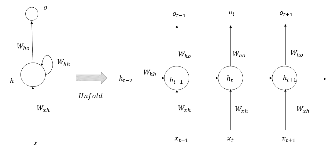
At each given time step, t, a memory state, h_t, is computed, based on the previous state, h_t-1, at step (t-1) and the input, x_t, at time step t. The new state, h_t, is used to predict the output, o_t, at step t. The equations governing RNNs are as follows:

If we are predicting the next word in a sentence, then the function f₂ is generally a softmax function over the words in the vocabulary. The function f₁ can be any activation function based on the problem at hand.

In an RNN, an output error in step t tries to correct the prediction in the previous time steps, generalized by k ∈ 1, 2, . . . t-1, by propagating the error in the previous time steps. This helps the RNN to learn about long dependencies between words that are far apart from each other. In practice, it isn't always possible to learn such long dependencies through RNN because of the vanishing and exploding gradient problems.

As you know, neural networks learn through gradient descent, and the relationship of a word in time step t with a word at a prior sequence step k can be learned through the gradient of the memory state with respect to the gradient of the memory state ∀ i. This is expressed in the following formula:

If the weight connection from the memory state at the sequence step k to the memory state at the sequence step (k+1) is given by u_ii ∈ W_hh, then the following is true:

In the preceding equation, is the total input to the memory state i at the time step (k+1), such that the following is the case:

Now that we have everything in place, it's easy to see why the vanishing gradient problem may occur in an RNN. From the preceding equations, (3) and (4), we get the following:

For RNNs, the function f₂ is generally sigmoid or tanh, which suffers from the saturation problem of having low gradients beyond a specified range of values for the input. Now, since the f₂ derivatives are multiplied with each other, the gradient can become zero if the input to the activation functions is operating at the saturation zone, even for relatively moderate values of (t-k). Even if the f₂ functions are not operating in the saturation zone, the gradients of the f₂ function for sigmoids are always less than 1, and so it is very difficult to learn distant dependencies between words in a sequence. Similarly, there might be exploding gradient problems stemming from the factor . Suppose that the distance between steps t and k is around 10, while the weight, u_ii, is around two. In such cases, the gradient would be magnified by a factor of two, 2¹⁰ = 1024, leading to the exploding gradient problem.

Long short-term memory (LSTM) cells

The vanishing gradient problem is taken care of, to a great extent, by a modified version of RNNs, called long short-term memory (LSTM) cells. The architectural diagram of a long short-term memory cell is as follows:

Figure 1.13: LSTM architecture

LSTM introduces the cell state, C_t, in addition to the memory state, h_t, that you already saw when learning about RNNs. The cell state is regulated by three gates: the forget gate, the update gate, and the output gate. The forget gate determines how much information to retain from the previous cell states, C_t-1, and its output is expressed as follows:

The output of the update gate is expressed as follows:

The potential new candidate cell state, , is expressed as follows:

Based on the previous cell state and the current potential cell state, the updated cell state output is given via the following:

Not all of the information of the cell state is passed on to the next step, and how much of the cell state should be released to the next step is determined by the output gate. The output of the output gate is given via the following:

Based on the current cell state and the output gate, the updated memory state passed on to the next step is given via the following:

Now comes the big question: How does LSTM avoid the vanishing gradient problem? The equivalent of in LSTM is given by , which can be expressed in a product form as follows:

Now, the recurrence in the cell state units is given by the following:

From this, we get the following:

As a result, the gradient expression, , becomes the following:

As you can see, if we can keep the forget cell state near one, the gradient will flow almost unattenuated, and the LSTM will not suffer from the vanishing gradient problem.

Most of the text-processing applications that we will look at in this book will use the LSTM version of RNNs.