Understanding probabilities
You can't escape the term probability in any machine learning literature, and it can be confusing as it can have different meanings in different contexts. Probability is often denoted as p in mathematical equations, and you see it everywhere in academic papers, tutorials, and blogs. Although it is a concept that is seemingly easy to understand, it can be quite confusing. This is because there are multiple different definitions and interpretations depending on the context. We will use some examples to clarify things. In this section, we will go over the use of probability in the following contexts:
- Distribution
- Belief
Probability distribution
Say we want to train a neural network to classify images of cats and dogs and that we found a dataset that contains 600 images of dogs and 400 images of cats. As you may be aware, the data will need to be shuffled before being fed into the neural network. Otherwise, if it sees only images of the same label in a minibatch, the network will get lazy and say all images have the same label without taking the effort to look hard and differentiate between them. If we sampled the dataset randomly, the probabilities could be written as follows:
pdata(dog) = 0.6
pdata(cat) = 0.4
The probabilities here refer to the data distribution. In this example, this refers to the ratio of the number of cat and dog images to the total number of images in the dataset. The probability here is static and will not change for a given dataset.
When training a deep neural network, the dataset is usually too big to fit into one batch, and we need to break it into multiple minibatches for one epoch. If the dataset is well shuffled, then the sampling distribution of the minibatches will resemble that of the data distribution. If the dataset is unbalanced, where some classes have a lot more images from one label than another, then the neural network may be biased toward predicting the images it sees more. This is a form of overfitting. We can therefore sample the data differently to give more weight to the less-represented classes. If we want to balance the classes in sampling, then the sampling probability becomes as follows:
psample(dog) = 0.5
psample(cat) = 0.5
Note
Probability distribution p(x) is the probability of the occurrence of a data point x. There are two common distributions that are used in machine learning. Uniform distribution is where every data point has the same chances of occurrence; this is what people normally imply when they say random sampling without specifying the distribution type. Gaussian distribution is another commonly used distribution. It is so common that people also call it normal distribution. The probabilities peak at the center (mean) and slowly decay on each side. Gaussian distribution also has nice mathematical properties that make it a favorite of mathematicians. We will see more of that in the next chapter.
Prediction confidence
After several hundred iterations, the model has finally finished training, and I can't wait to test the new model with an image. The model outputs the following probabilities:
p(dog) = 0.6
p(cat) = 0.4
Wait, is the AI telling me that this animal is a mixed-breed with 60% dog genes and 40% cat inheritance? Of course not!
Here, the probabilities no longer refer to distributions; instead, they tell us how confident we can be about the predictions, or in other words, how strongly we can believe in the output. Now, this is no longer something you quantify by counting occurrences. If you are absolutely sure that something is a dog, you can put p(dog) = 1.0 and p(cat) = 0.0. This is known as Bayesian probability.
Note
The traditional statistics approach sees probability as the chances of the occurrence of an event, for example, the chances of a baby being a certain sex. There has been great debate in the wider statistical field on whether the frequentist or Bayesian method is better, which is beyond the scope of this book. However, the Bayesian method is probably more important in deep learning and engineering. It has been used to develop many important algorithms, including Kalman filtering to track rocket trajectory. When calculating the projection of a rocket's trajectory, the Kalman filter uses information from both the global positioning system (GPS) and speed sensor. Both sets of data are noisy, but GPS data is less reliable initially (meaning less confidence), and hence this data is given less weight in the calculation. We don't need to learn the Bayesian theorem in this book; it's enough to understand that probability can be viewed as a confidence score rather than as frequency. Bayesian probability has also recently been used in searching for hyperparameters for deep neural networks.
We have now clarified two main types of probabilities commonly used in general machine learning – distribution and confidence. From now on, we will assume that probability means probability distribution rather than confidence. Next, we will look at a distribution that plays an exceptionally important role in image generation – pixel distribution.
The joint probability of pixels
Take a look at the following pictures – can you tell whether they are of dogs or cats? How do you think the classifier will produce the confidence score?
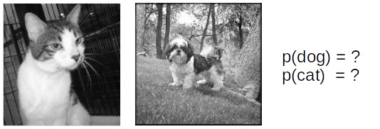
Figure 1.1 – Pictures of a cat and a dog
Are either of these pictures of dogs or cats? Well, the answer is pretty obvious, but at the same time it's not important to what we are going to talk about. When you looked at the pictures, you probably thought in your mind that the first picture was of a cat and the second picture was of a dog. We see the picture as a whole, but that is not what the computer sees. The computer sees pixels.
Note
A pixel is the smallest spatial unit in digital image, and it represents a single color. You cannot have a pixel where half is black and the other half is white. The most commonly used color scheme is 8-bit RGB, where a pixel is made up of three channels named R (red), G (green), and B (blue). Their values range from 0 to 255 (255 being the highest intensity). For example, a black pixel has a value of [0, 0, 0], while a white pixel is [255, 255, 255].
The simplest way to describe the pixel distribution of an image is by counting the number of pixels that have different intensity levels from 0 to 255; you can visualize this by plotting a histogram. It is a common tool in digital photography to look at a histogram of separate R, G, and B channels to understand the color balance. Although this can provide some information to us – for example, an image of sky is likely to have many blue pixels, so a histogram may reliably tell us something about that – histograms do not tell us how pixels relate to each other. In other words, a histogram does not contain spatial information, that is, how far a blue pixel is from another blue pixel. We will need a better measure for this kind of thing.
Instead of saying p(x), where x is a whole image, we can define x as x1, x2, x3,… xn. Now, p(x) can be defined as the joint probability of pixels p(x1, x2, x3,… xn), where n is the number of pixels and each pixel is separated by a comma.
We will use the following images to illustrate what we mean by joint probability. The following are three images with 2 x 2 pixels that contain binary values, where 0 is black and 1 is white. We will call the top-left pixel x1, the top-right pixel x2, the bottom-left pixel x3, and the bottom-right pixel x4:

Figure 1.2 – Images with 2 x 2 pixels
We first calculate p(x1 = white) by counting the number of white x1 and dividing it by the total number of the image. Then, we do the same for x2, as follows:
p(x1 = white) = 2 / 3
p(x2 = white) = 0 / 3
Now we say that p(x1) and p(x2) are independent of each other because we calculated them separately. If we calculate the joint probability where both x1 and x2 are black, we get the following:
p(x1 = black, x2 = black) = 0 / 3
We can then calculate the complete joint probability of these two pixels as follows:
p(x1 = black, x2 = white) = 0 / 3
p(x1 = white, x2 = black) = 3 / 3
p(x1 = white, x2 = white) = 0 / 3
We'll need to do the same steps 16 times to calculate the complete joint probability of p(x1, x2, x3, x4). Now, we could fully describe the pixel distribution and use that to calculate the marginal distribution, as in p(x1, x2, x3) or p(x1). However, the calculations required for the joint distribution increase exponentially for RGB values where each pixel has 256 x 256 x 256 = 16,777,216 possibilities. This is where deep neural networks come to the rescue. A neural network can be trained to learn a pixel data distribution Pdata. Hence, a neural network is our probability model Pmodel.
Important Note
The notations we will use in this book are as follows: capital X for the dataset, lowercase x for image sampled from the dataset, and lowercase with subscript xi for the pixel.
The purpose of image generation is to generate an image that has a pixel distribution p(x) that resembles p(X). For example, an image dataset of oranges will have a high probability of lots of occurrences of orange pixels that are distributed close to each other in a circle. Therefore, before generating image, we will first build a probability model pmodel(x) from real data pdata(X). After that, we generate images by drawing a sample from pmodel(x).


