Search icon CANCEL
Subscription
0
Cart icon
Your Cart (0 item)
Close icon
You have no products in your basket yet
Arrow left icon
Explore Products
Best Sellers
New Releases
Books
Videos
Audiobooks
Learning Hub
Free Learning
Arrow right icon
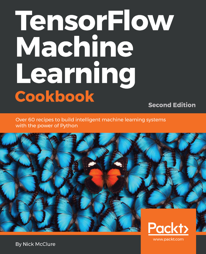
TensorFlow Machine Learning Cookbook

TensorFlow Machine Learning Cookbook: Over 60 recipes to build intelligent machine learning systems with the power of Python , Second Edition

Arrow left icon
Profile Icon Sujit Pal Profile Icon Nick McClure
Arrow right icon
R$217.99
Full star icon Full star icon Empty star icon Empty star icon Empty star icon 2 (3 Ratings)
Paperback Aug 2018 422 pages 2nd Edition
eBook
R$49.99 R$173.99
Paperback
R$217.99
Subscription
Free Trial
Renews at R$50p/m
eBook
R$49.99 R$173.99
Paperback
R$217.99
Subscription
Free Trial
Renews at R$50p/m

What do you get with Print?

Product feature icon Instant access to your digital eBook copy whilst your Print order is Shipped
Product feature icon Paperback book shipped to your preferred address
Product feature icon Download this book in EPUB and PDF formats
Product feature icon Access this title in our online reader with advanced features
Product feature icon DRM FREE - Read whenever, wherever and however you want
OR
Modal Close icon
Payment Processing...
tick Completed

Shipping Address

Billing Address

Shipping Methods
Table of content icon View table of contents Preview book icon Preview Book

TensorFlow Machine Learning Cookbook

Getting Started with TensorFlow

In this chapter, we will cover some basic recipes in order to understand how TensorFlow works and how to access data for this book and additional resources.

By the end of this chapter, you should have knowledge of the following:

  • How TensorFlow works
  • Declaring variables and tensors
  • Using placeholders and variables
  • Working with matrices
  • Declaring operations
  • Implementing activation functions
  • Working with data sources
  • Additional resources

Introduction

Google's TensorFlow engine has a unique way of solving problems. This unique way allows us to solve machine learning problems very efficiently. Machine learning is used in almost all areas of life and work, but some of the more famous areas are computer vision, speech recognition, language translations, healthcare, and many more. We will cover the basic steps to understand how TensorFlow operates and eventually build up to production code techniques later in this book. These fundamentals are important to understanding recipes for the rest of this book.

How TensorFlow works

At first, computation in TensorFlow may seem needlessly complicated. But there is a reason for it: because of how TensorFlow treats computation, developing more complicated algorithms is relatively easy. This recipe will guide us through the pseudocode of a TensorFlow algorithm.

Getting ready

Currently, TensorFlow is supported on Linux, macOS, and Windows. The code for this book has been created and run on a Linux system, but should run on any other system as well. The code for the book is available on GitHub at https://github.com/nfmcclure/tensorflow_cookbook as well as the Packt repository: https://github.com/PacktPublishing/TensorFlow-Machine-Learning-Cookbook-Second-Edition.

Throughout this book, we will only concern ourselves with the Python library wrapper of TensorFlow, although most of the original core code for TensorFlow is written in C++. This book will use Python 3.6+ (https://www.python.org) and TensorFlow 1.10.0+ (https://www.tensorflow.org). While TensorFlow can run on the CPU, most algorithms run faster if processed on the GPU, and it is supported on graphics cards with Nvidia Compute Capability v4.0+ (v5.1 recommended).

Popular GPUs for TensorFlow are Nvidia Tesla architectures and Pascal architectures with at least 4 GB of video RAM. To run on a GPU, you will also need to download and install the Nvidia CUDA toolkit as well as version 5.x+ (https://developer.nvidia.com/cuda-downloads).

Some of the recipes in this chapter will rely on a current installation of the SciPy, NumPy, and scikit-learn Python packages. These accompanying packages are also included in the Anaconda package (https://www.continuum.io/downloads).

How to do it...

Here, we will introduce the general flow of TensorFlow algorithms. Most recipes will follow this outline:

  1. Import or generate dataset: All of our machine learning algorithms will depend on datasets. In this book, we will either generate data or use an outside source of datasets. Sometimes, it is better to rely on generated data because we just want to know the expected outcome. Most of the time, we will access public datasets for the given recipe. The details on accessing these datasets are in additional resources, section 8 of this chapter.
  2. Transform and normalize data: Normally, input datasets do not come into the picture. TensorFlow expects that we need to transform TensorFlow so that they get the accepted shape. The data is usually not in the correct dimension or type that our algorithms expect. We will have to transform our data before we can use it. Most algorithms also expect normalized data and we will look at this here as well. TensorFlow has built-in functions that can normalize data for you, as follows:
import tensorflow as tf
data = tf.nn.batch_norm_with_global_normalization(...)
  1. Partition the dataset into train, test, and validation sets: We generally want to test our algorithms on different sets that we have trained on. Also, many algorithms require hyperparameter tuning, so we set aside a validation set for determining the best set of hyperparameters.
  2. Set algorithm parameters (hyperparameters): Our algorithms usually have a set of parameters that we hold constant throughout the procedure. For example, this can be the number of iterations, the learning rate, or other fixed parameters of our choosing. It is considered good practice to initialize these together so that the reader or user can easily find them, as follows:
learning_rate = 0.01 
batch_size = 100 
iterations = 1000
  1. Initialize variables and placeholders: TensorFlow depends on knowing what it can and cannot modify. TensorFlow will modify/adjust the variables (model weights/biases) during optimization to minimize a loss function. To accomplish this, we feed in data through placeholders. We need to initialize both variables and placeholders with size and type so that TensorFlow knows what to expect. TensorFlow also needs to know the type of data to expect. For most of this book, we will use float32. TensorFlow also provides float64 and float16. Note that more bytes used for precision results in slower algorithms, but less used results in less precision. See the following code:
a_var = tf.constant(42) 
x_input = tf.placeholder(tf.float32, [None, input_size]) 
y_input = tf.placeholder(tf.float32, [None, num_classes]) 
  1. Define the model structure: After we have the data, and have initialized our variables and placeholders, we have to define the model. This is done by building a computational graph. We will talk more in depth about computational graphs in the Operations in a Computational Graph TensorFlow recipe in Chapter 2, The TensorFlow Way. The model for this example will be a linear model ():
y_pred = tf.add(tf.mul(x_input, weight_matrix), b_matrix) 
  1. Declare the loss functions: After defining the model, we must be able to evaluate the output. This is where we declare the loss function. The loss function is very important as it tells us how far off our predictions are from the actual values. The different types of loss functions are explored in greater detail in the Implementing Back Propagation recipe in Chapter 2, The TensorFlow Way. Here, we implement the mean squared error for n-points, that is, :
loss = tf.reduce_mean(tf.square(y_actual - y_pred)) 
  1. Initialize and train the model: Now that we have everything in place, we need to create an instance of our graph, feed in the data through the placeholders, and let TensorFlow change the variables to better predict our training data. Here is one way to initialize the computational graph:
with tf.Session(graph=graph) as session: 
... 
session.run(...) 
... 
Note that we can also initiate our graph with:
session = tf.Session(graph=graph) session.run(...)
  1. Evaluate the model: Once we have built and trained the model, we should evaluate the model by looking at how well it does with new data through some specified criteria. We evaluate on the train and test set and these evaluations will allow us to see if the model is under overfitting. We will address this in later recipes.
  2. Tune hyperparameters: Most of the time, we will want to go back and change some of the hyperparameters based on the model's performance. We then repeat the previous steps with different hyperparameters and evaluate the model on the validation set.
  3. Deploy/predict new outcomes: It is also important to know how to make predictions on new and unseen data. We can do this with all of our models once we have them trained.

How it works...

In TensorFlow, we have to set up the data, variables, placeholders, and model before we can tell the program to train and change the variables to improve predictions. TensorFlow accomplishes this through computational graphs. These computational graphs are directed graphs with no recursion, which allows for computational parallelism. To do this, we need to create a loss function for TensorFlow to minimize. TensorFlow accomplishes this by modifying the variables in the computational graph. TensorFlow knows how to modify the variables because it keeps track of the computations in the model and automatically computes the variable gradients (how to change each variable) to minimize the loss. Because of this, we can see how easy it can be to make changes and try different data sources.

See also

Declaring variables and tensors

Tensors are the primary data structure that TensorFlow uses to operate on the computational graph. We can declare these tensors as variables and/or feed them in as placeholders. To do this, first, we must learn how to create tensors.

A tensor is a mathematical term that refers to generalized vectors or matrices. If vectors are one-dimensional and matrices are two-dimensional, a tensor is n-dimensional (where n could be 1, 2, or even larger).

Getting ready

When we create a tensor and declare it as a variable, TensorFlow creates several graph structures in our computation graph. It is also important to point out that just by creating a tensor, TensorFlow is not adding anything to the computational graph. TensorFlow does this only after running an operation to initialize the variables. See the next section, on variables and placeholders, for more information.

How to do it...

Here, we will cover the main ways that we can create tensors in TensorFlow:

1. Fixed tensors:

    • In the following code, we are creating a zero-filled tensor:
zero_tsr = tf.zeros([row_dim, col_dim])
    • In the following code, we are creating a one-filled tensor:
ones_tsr = tf.ones([row_dim, col_dim]) 
    • In the following code, we are creating a constant-filled tensor:
filled_tsr = tf.fill([row_dim, col_dim], 42) 
    • In the following code, we are creating a tensor out of an existing constant:
constant_tsr = tf.constant([1,2,3])
Note that the tf.constant() function can be used to broadcast a value into an array, mimicking the behavior of tf.fill() by writing tf.constant(42, [row_dim, col_dim]).
  1. Tensors of similar shape: We can also initialize variables based on the shape of other tensors, as follows:
zeros_similar = tf.zeros_like(constant_tsr) 
ones_similar = tf.ones_like(constant_tsr) 
Note that since these tensors depend on prior tensors, we must initialize them in order. Attempting to initialize all the tensors all at once will result in an error. See the There's more... subsection at the end of the next section, on variables and placeholders.
  1. Sequence tensors: TensorFlow allows us to specify tensors that contain defined intervals. The following functions behave very similarly to the NumPy's linspace() outputs and range() outputs. See the following function:
linear_tsr = tf.linspace(start=0, stop=1, start=3) 

The resultant tensor has a sequence of [0.0, 0.5, 1.0]. Note that this function includes the specified stop value. See the following function for more information:

integer_seq_tsr = tf.range(start=6, limit=15, delta=3) 

The result is the sequence [6, 9, 12]. Note that this function does not include the limit value.

  1. Random tensors: The following generated random numbers are from a uniform distribution:
randunif_tsr = tf.random_uniform([row_dim, col_dim], minval=0, maxval=1) 

Note that this random uniform distribution draws from the interval that includes the minval but not the maxval (minval <= x < maxval).

To get a tensor with random draws from a normal distribution, you can run the following code:

randnorm_tsr = tf.random_normal([row_dim, col_dim], mean=0.0, stddev=1.0) 

There are also times where we want to generate normal random values that are assured within certain bounds. The truncated_normal() function always picks normal values within two standard deviations of the specified mean:

runcnorm_tsr = tf.truncated_normal([row_dim, col_dim], mean=0.0, stddev=1.0) 

We might also be interested in randomizing entries of arrays. To accomplish this, there are two functions that can help us: random_shuffle() and random_crop(). The following code performs this:

shuffled_output = tf.random_shuffle(input_tensor) 
cropped_output = tf.random_crop(input_tensor, crop_size) 

Later on in this book, we will be interested in randomly cropping images of size (height, width, 3) where there are three color spectrums. To fix a dimension in the cropped_output, you must give it the maximum size in that dimension:

cropped_image = tf.random_crop(my_image, [height/2, width/2, 3]) 

How it works...

Once we have decided how to create the tensors, we may also create the corresponding variables by wrapping the tensor in the Variable() function, as follows (more on this in the next section):

my_var = tf.Variable(tf.zeros([row_dim, col_dim])) 

There's more...

We are not limited to the built-in functions: we can convert any NumPy array into a Python list, or a constant into a tensor using the convert_to_tensor() function. Note that this function also accepts tensors as an input in case we wish to generalize a computation inside a function.

Using placeholders and variables

Placeholders and variables are key tools in with regard to using computational graphs in TensorFlow. We must understand the difference between them and when to best use them to our advantage.

Getting ready

One of the most important distinctions to make with data is whether it is a placeholder or a variable. Variables are the model parameters of the algorithm, and TensorFlow keeps track of how to change these to optimize the algorithm. Placeholders are objects that allow you to feed in data of a specific type and shape, or that depend on the results of the computational graph, such as the expected outcome of a computation.

How to do it...

The main way to create a variable is by using the Variable() function, which takes a tensor as an input and outputs a variable. This is only the declaration, and we still need to initialize the variable. Initializing is what puts the variable with the corresponding methods on the computational graph. Here is an example of creating and initializing a variable:

my_var = tf.Variable(tf.zeros([2,3])) 
sess = tf.Session() 
initialize_op = tf.global_variables_initializer() 
sess.run(initialize_op) 

To see what the computational graph looks like after creating and initializing a variable, see the following part of this recipe. Placeholders are just holding the position for data to be fed into the graph. Placeholders get data from a feed_dict argument in the session. To put a placeholder into the graph, we must perform at least one operation on the placeholder. In the following code snippet, we initialize the graph, declare x to be a placeholder (of a predefined size), and define y as the identity operation on x, which just returns x. We then create data to feed into the x placeholder and run the identity operation. The code is shown here, and the resultant graph is in the following section:

sess = tf.Session() 
x = tf.placeholder(tf.float32, shape=[2,2]) 
y = tf.identity(x) 
x_vals = np.random.rand(2,2) 
sess.run(y, feed_dict={x: x_vals}) 
# Note that sess.run(x, feed_dict={x: x_vals}) will result in a self-referencing error. 
It is worth noting that TensorFlow will not return a self-referenced placeholder in the feed dictionary. In other words, running sess.run(x, feed_dict={x: x_vals}) in the following graph will return an error.

How it works...

The computational graph of initializing a variable as a tensor of zeros is shown in the following diagram:

Figure 1: Variable

Here, we can see what the computational graph looks like in detail with just one variable, initialized all to zeros. The grey shaded region is a very detailed view of the operations and constants that were involved. The main computational graph with less detail is the smaller graph outside of the grey region in the upper-right corner. For more details on creating and visualizing graphs, see the first section of Chapter 10, Taking TensorFlow to Production. Similarly, the computational graph of feeding a NumPy array into a placeholder can be seen in the following diagram:

Figure 2: The computational graph of an initialized placeholder

The grey shaded region is a very detailed view of the operations and constants that were involved. The main computational graph with less detail is the smaller graph outside of the grey region in the upper-right corner.

There's more...

During the run of the computational graph, we have to tell TensorFlow when to initialize the variables we have created. While each variable has an initializer method, the most common way to do this is with the helper function, that is, global_variables_initializer(). This function creates an operation in the graph that initializes all the variables we have created, as follows:

initializer_op = tf.global_variables_initializer() 

But if we want to initialize a variable based on the results of initializing another variable, we have to initialize variables in the order we want, as follows:

sess = tf.Session() 
first_var = tf.Variable(tf.zeros([2,3])) 
sess.run(first_var.initializer) 
second_var = tf.Variable(tf.zeros_like(first_var)) 
# 'second_var' depends on the 'first_var'
sess.run(second_var.initializer)

Working with matrices

Understanding how TensorFlow works with matrices is very important in understanding the flow of data through computational graphs.

It is worth emphasizing the importance of matrices in machine learning (and mathematics in general). Most machine learning algorithms are computationally expressed as matrix operations. This book does not cover the mathematical background on matrix properties and matrix algebra (linear algebra), so the reader is strongly encouraged to learn enough about matrices to be comfortable with matrix algebra.

Getting ready

Many algorithms depend on matrix operations. TensorFlow gives us easy-to-use operations to perform such matrix calculations. For all of the following examples, we first create a graph session by running the following code:

import tensorflow as tf 
sess = tf.Session() 

How to do it...

We will proceed with the recipe as follows:

  1. Creating matrices: We can create two-dimensional matrices from NumPy arrays or nested lists, as we described in the Creating and using tensors recipe. We can also use the tensor creation functions and specify a two-dimensional shape for functions such as zeros(), ones(), truncated_normal(), and so on. TensorFlow also allows us to create a diagonal matrix from a one-dimensional array or list with the diag() function, as follows:
identity_matrix = tf.diag([1.0, 1.0, 1.0]) 
A = tf.truncated_normal([2, 3]) 
B = tf.fill([2,3], 5.0) 
C = tf.random_uniform([3,2]) 
D = tf.convert_to_tensor(np.array([[1., 2., 3.],[-3., -7., -1.],[0., 5., -2.]])) 
print(sess.run(identity_matrix)) 
[[ 1.  0.  0.] 
 [ 0.  1.  0.] 
 [ 0.  0.  1.]] 
print(sess.run(A)) 
[[ 0.96751703  0.11397751 -0.3438891 ] 
 [-0.10132604 -0.8432678   0.29810596]] 
print(sess.run(B)) 
[[ 5.  5.  5.] 
 [ 5.  5.  5.]] 
print(sess.run(C)) 
[[ 0.33184157  0.08907614] 
 [ 0.53189191  0.67605299] 
 [ 0.95889051 0.67061249]] 
print(sess.run(D)) 
[[ 1.  2.  3.] 
 [-3. -7. -1.] 
 [ 0.  5. -2.]] 
Note that if we were to run sess.run(C) again, we would reinitialize the random variables and end up with different random values.
  1. Addition, subtraction, and multiplication: To add, subtract, or multiply matrices of the same dimension, TensorFlow uses the following function:
print(sess.run(A+B)) 
[[ 4.61596632  5.39771316  4.4325695 ] 
 [ 3.26702736  5.14477345  4.98265553]] 
print(sess.run(B-B)) 
[[ 0.  0.  0.] 
 [ 0.  0.  0.]] 
Multiplication 
print(sess.run(tf.matmul(B, identity_matrix))) 
[[ 5.  5.  5.] 
 [ 5.  5.  5.]] 

It is important to note that the matmul() function has arguments that specify whether or not to transpose the arguments before multiplication or whether each matrix is sparse.

Note that matrix division is not explicitly defined. While many define matrix division as multiplying by the inverse, it is fundamentally different compared to real-numbered division.
  1. The transpose: Transpose a matrix (flip the columns and rows) as follows:
print(sess.run(tf.transpose(C))) 
[[ 0.67124544  0.26766731  0.99068872] 
 [ 0.25006068  0.86560275  0.58411312]] 

Again, it is worth mentioning that reinitializing gives us different values than before.

  1. Determinant: To calculate the determinant, use the following:
print(sess.run(tf.matrix_determinant(D))) 
-38.0 
  1. Inverse: To find the inverse of a square matrix, see the following:
print(sess.run(tf.matrix_inverse(D))) 
[[-0.5        -0.5        -0.5       ] 
 [ 0.15789474  0.05263158  0.21052632] 
 [ 0.39473684  0.13157895  0.02631579]] 
The inverse method is based on the Cholesky decomposition, only if the matrix is symmetric positive definite. If the matrix is not symmetric positive definite then it is based on the LU decomposition.
  1. Decompositions: For the Cholesky decomposition, use the following:
print(sess.run(tf.cholesky(identity_matrix))) 
[[ 1.  0.  1.] 
 [ 0.  1.  0.] 
 [ 0.  0.  1.]] 
  1. Eigenvalues and eigenvectors: For eigenvalues and eigenvectors, use the following code:
print(sess.run(tf.self_adjoint_eig(D)) 
[[-10.65907521  -0.22750691   2.88658212] 
 [  0.21749542   0.63250104  -0.74339638] 
 [  0.84526515   0.2587998    0.46749277] 
 [ -0.4880805    0.73004459   0.47834331]] 

Note that the self_adjoint_eig() function outputs the eigenvalues in the first row and the subsequent vectors in the remaining vectors. In mathematics, this is known as the eigendecomposition of a matrix.

How it works...

TensorFlow provides all the tools for us to get started with numerical computations and adding such computations to our graphs. This notation might seem quite heavy for simple matrix operations. Remember that we are adding these operations to the graph and telling TensorFlow which tensors to run through those operations. While this might seem verbose now, it helps us understand the notation in later chapters when this way of computation will make it easier to accomplish our goals.

Declaring operations

Now, we must learn what other operations we can add to a TensorFlow graph.

Getting ready

Besides the standard arithmetic operations, TensorFlow provides us with more operations that we should be aware of and how to use them before proceeding. Again, we can create a graph session by running the following code:

import tensorflow as tf 
sess = tf.Session() 

How to do it...

TensorFlow has the standard operations on tensors, that is, add(), sub(), mul(), and div(). Note that all of the operations in this section will evaluate the inputs element-wise, unless specified otherwise:

  1. TensorFlow provides some variations of div() and the relevant functions.
  2. It is worth mentioning that div() returns the same type as the inputs. This means that it really returns the floor of the division (akin to Python 2) if the inputs are integers. To return the Python 3 version, which casts integers into floats before dividing and always returning a float, TensorFlow provides the truediv() function, as follows:
print(sess.run(tf.div(3, 4))) 
0 
print(sess.run(tf.truediv(3, 4))) 
0.75 
  1. If we have floats and want integer division, we can use the floordiv() function. Note that this will still return a float, but it will be rounded down to the nearest integer. This function is as follows:
print(sess.run(tf.floordiv(3.0,4.0))) 
0.0 
  1. Another important function is mod(). This function returns the remainder after division. It is as follows:
print(sess.run(tf.mod(22.0, 5.0))) 
2.0 
  1. The cross product between two tensors is achieved by the cross() function. Remember that the cross product is only defined for two three-dimensional vectors, so it only accepts two three-dimensional tensors. The following code illustrates this use:
print(sess.run(tf.cross([1., 0., 0.], [0., 1., 0.]))) 
[ 0.  0.  1.0]

  1. Here is a compact list of the more common math functions. All of these functions operate element-wise:

abs()

Absolute value of one input tensor

ceil()

Ceiling function of one input tensor

cos()

Cosine function of one input tensor

exp()

Base e exponential of one input tensor

floor()

Floor function of one input tensor

inv()

Multiplicative inverse (1/x) of one input tensor

log()

Natural logarithm of one input tensor

maximum()

Element-wise max of two tensors

minimum()

Element-wise min of two tensors

neg()

Negative of one input tensor

pow()

The first tensor raised to the second tensor element-wise

round()

Rounds one input tensor

rsqrt()

One over the square root of one tensor

sign()

Returns -1, 0, or 1, depending on the sign of the tensor

sin()

Sine function of one input tensor

sqrt()

Square root of one input tensor

square()

Square of one input tensor

  1. Specialty mathematical functions: There are some special math functions that get used in machine learning that are worth mentioning, and TensorFlow has built-in functions for them. Again, these functions operate element-wise, unless specified otherwise:

digamma()

Psi function, the derivative of the lgamma() function

erf()

Gaussian error function, element-wise, of one tensor

erfc()

Complementary error function of one tensor

igamma()

Lower regularized incomplete gamma function

igammac()

Upper regularized incomplete gamma function

lbeta()

Natural logarithm of the absolute value of the beta function

lgamma()

Natural logarithm of the absolute value of the gamma function

squared_difference()

Computes the square of the differences between two tensors

How it works...

It is important to know which functions are available to us so that we can add them to our computational graphs. We will mainly be concerned with the preceding functions. We can also generate many different custom functions as compositions of the preceding, as follows:

# Tangent function (tan(pi/4)=1) 
print(sess.run(tf.tan(3.1416/4.)))
1.0 

There's more...

If we wish to add other operations to our graphs that are not listed here, we must create our own from the preceding functions. Here is an example of an operation that wasn't used previously that we can add to our graph. We chose to add a custom polynomial function, , using the following code:

def custom_polynomial(value): 
    return tf.sub(3 * tf.square(value), value) + 10
print(sess.run(custom_polynomial(11))) 362

Implementing activation functions

Activation functions are the key for neural networks to approximate non-linear outputs and adapt to non-linear features. They introduce non-linear operations into neural networks. If we are careful as to which activation functions are selected and where we put them, they are very powerful operations that we can tell TensorFlow to fit and optimize.

Getting ready

When we start to use neural networks, we will use activation functions regularly because activation functions are an essential part of any neural network. The goal of an activation function is just to adjust weight and bias. In TensorFlow, activation functions are non-linear operations that act on tensors. They are functions that operate in a similar way to the previous mathematical operations. Activation functions serve many purposes, but the main concept is that they introduce a non-linearity into the graph while normalizing the outputs. Start a TensorFlow graph with the following commands:

import tensorflow as tf 
sess = tf.Session() 

How to do it...

The activation functions live in the neural network (nn) library in TensorFlow. Besides using built-in activation functions, we can also design our own using TensorFlow operations. We can import the predefined activation functions (import tensorflow.nn as nn) or be explicit and write nn in our function calls. Here, we choose to be explicit with each function call:

  1. The rectified linear unit, known as ReLU, is the most common and basic way to introduce non-linearity into neural networks. This function is just called max(0,x). It is continuous, but not smooth. It appears as follows:
print(sess.run(tf.nn.relu([-3., 3., 10.]))) 
[  0.  3.  10.] 
  1. There are times where we will want to cap the linearly increasing part of the preceding ReLU activation function. We can do this by nesting the max(0,x) function into a min() function. The implementation that TensorFlow has is called the ReLU6 function. This is defined as min(max(0,x),6). This is a version of the hard-sigmoid function and is computationally faster, and does not suffer from vanishing (infinitesimally near zero) or exploding values. This will come in handy when we discuss deeper neural networks in Chapter 8, Convolutional Neural Networks, and Chapter 9, Recurrent Neural Networks. It appears as follows:
print(sess.run(tf.nn.relu6([-3., 3., 10.]))) 
[ 0. 3. 6.]
  1. The sigmoid function is the most common continuous and smooth activation function. It is also called a logistic function and has the form . The sigmoid function is not used very often because of its tendency to zero-out the backpropagation terms during training. It appears as follows:
print(sess.run(tf.nn.sigmoid([-1., 0., 1.]))) 
[ 0.26894143  0.5         0.7310586 ] 
We should be aware that some activation functions are not zero-centered, such as the sigmoid. This will require us to zero-mean data prior to using it in most computational graph algorithms.
  1. Another smooth activation function is the hyper tangent. The hyper tangent function is very similar to the sigmoid except that instead of having a range between 0 and 1, it has a range between -1 and 1. This function has the form of the ratio of the hyperbolic sine over the hyperbolic cosine. Another way to write this is . This activation function is as follows:
print(sess.run(tf.nn.tanh([-1., 0., 1.]))) 
[-0.76159418  0.         0.76159418 ] 
  1. The softsign function also gets used as an activation function. The form of this function is . The softsign function is supposed to be a continuous (but not smooth) approximation to the sign function. See the following code:
print(sess.run(tf.nn.softsign([-1., 0., -1.]))) 
[-0.5  0.   0.5] 
  1. Another function, the softplus function, is a smooth version of the ReLU function. The form of this function is . It appears as follows:
print(sess.run(tf.nn.softplus([-1., 0., -1.]))) 
[ 0.31326166  0.69314718  1.31326163] 
The softplus function goes to infinity as the input increases, whereas the softsign function goes to 1. As the input gets smaller, however, the softplus function approaches zero and the softsign function goes to -1.
  1. The Exponential Linear Unit (ELU) is very similar to the softplus function except that the bottom asymptote is -1 instead of 0. The form is if x < 0 else x. It appears as follows:
print(sess.run(tf.nn.elu([-1., 0., -1.]))) 
[-0.63212055  0.          1.        ] 

How it works...

These activation functions are ways that we can introduce non-linearities in neural networks or other computational graphs in the future. It is important to note where in our network we are using activation functions. If the activation function has a range between 0 and 1 (sigmoid), then the computational graph can only output values between 0 and 1. If the activation functions are inside and hidden between nodes, then we want to be aware of the effect that the range can have on our tensors as we pass them through. If our tensors were scaled to have a mean of zero, we will want to use an activation function that preserves as much variance as possible around zero. This would imply that we want to choose an activation function such as the hyperbolic tangent (tanh) or the softsign. If the tensors are all scaled to be positive, then we would ideally choose an activation function that preserves variance in the positive domain.

There's more...

Here are two graphs that illustrate the different activation functions. The following graphs show the ReLU, ReLU6, softplus, exponential LU, sigmoid, softsign, and hyperbolic tangent functions:

Figure 3: Activation functions of softplus, ReLU, ReLU6, and exponential LU

Here, we can see four of the activation functions: softplus, ReLU, ReLU6, and exponential LU. These functions flatten out to the left of zero and linearly increase to the right of zero, with the exception of ReLU6, which has a maximum value of six:

Figure 4: Sigmoid, hyperbolic tangent (tanh), and softsign activation function

Here are the sigmoid, hyperbolic tangent (tanh), and softsign activation functions. These activation functions are all smooth and have a S n shape. Note that there are two horizontal asymptotes for these functions.

Working with data sources

For most of this book, we will rely on the use of datasets to fit machine learning algorithms. This section has instructions on how to access each of these datasets through TensorFlow and Python.

Some of the data sources rely on the maintenance of outside websites so that you can access the data. If these websites change or remove this data, then some of the following code in this section may need to be updated. You may find the updated code at the author's GitHub page: https://github.com/nfmcclure/tensorflow_cookbook.

Getting ready

In TensorFlow, some of the datasets that we will use are built into Python libraries, some will require a Python script to download, and some will be manually downloaded through the internet. Almost all of these datasets will require an active internet connection so that you can retrieve them.

How to do it...

  1. Iris data: This dataset is arguably the most classic dataset used in machine learning and maybe all of statistics. It is a dataset that measures sepal length, sepal width, petal length, and petal width of three different types of iris flowers: Iris setosa, Iris virginica, and Iris versicolor. There are 150 measurements overall, which means that there are 50 measurements of each species. To load the dataset in Python, we will use scikit-learn's dataset function, as follows:
from sklearn import datasets 
iris = datasets.load_iris() 
print(len(iris.data)) 
150 
print(len(iris.target)) 
150 
print(iris.data[0]) # Sepal length, Sepal width, Petal length, Petal width 
[ 5.1 3.5 1.4 0.2] 
print(set(iris.target)) # I. setosa, I. virginica, I. versicolor 
{0, 1, 2} 
  1. Birth weight data: This data was originally from Baystate Medical Center, Springfield, Mass 1986 (1). This dataset contains the measure of child birth weight and other demographic and medical measurements of the mother and family history. There are 189 observations of eleven variables. The following code shows you how you can access this data in Python:
import requests
birthdata_url = 'https://github.com/nfmcclure/tensorflow_cookbook/raw/master/01_Introduction/07_Working_with_Data_Sources/birthweight_data/birthweight.dat'
birth_file = requests.get(birthdata_url)
birth_data = birth_file.text.split('\r\n')
birth_header = birth_data[0].split('\t')
birth_data = [[float(x) for x in y.split('\t') if len(x)>=1] for y in birth_data[1:] if len(y)>=1]
print(len(birth_data)) 189 print(len(birth_data[0])) 9

  1. Boston Housing data: Carnegie Mellon University maintains a library of datasets in their StatLib Library. This data is easily accessible via The University of California at Irvine's machine learning Repository (https://archive.ics.uci.edu/ml/index.php). There are 506 observations of house worth, along with various demographic data and housing attributes (14 variables). The following code shows you how to access this data in Python, via the Keras library:
from keras.datasets import boston_housing
(x_train, y_train), (x_test, y_test) = boston_housing.load_data()
housing_header = ['CRIM', 'ZN', 'INDUS', 'CHAS', 'NOX', 'RM', 'AGE', 'DIS', 'RAD', 'TAX', 'PTRATIO', 'B', 'LSTAT', 'MEDV'] print(x_train.shape[0]) 404 print(x_train.shape[1]) 13
  1. MNIST handwriting data: The MNIST (Mixed National Institute of Standards and Technology) dataset is a subset of the larger NIST handwriting database. The MNIST handwriting dataset is hosted on Yann LeCun's website (https://yann.lecun.com/exdb/mnist/). It is a database of 70,000 images of single-digit numbers (0-9) with about 60,000 annotated for a training set and 10,000 for a test set. This dataset is used so often in image recognition that TensorFlow provides built-in functions to access this data. In machine learning, it is also important to provide validation data to prevent overfitting (target leakage). Because of this, TensorFlow sets aside 5,000 images of the train set into a validation set. The following code shows you how to access this data in Python:
from tensorflow.examples.tutorials.mnist import input_data 
mnist = input_data.read_data_sets("MNIST_data/"," one_hot=True) 
print(len(mnist.train.images)) 
55000 
print(len(mnist.test.images)) 
10000 
print(len(mnist.validation.images)) 
5000 
print(mnist.train.labels[1,:]) # The first label is a 3 
[ 0.  0.  0.  1.  0.  0.  0.  0.  0.  0.] 
  1. Spam-ham text data. UCI's machine learning dataset library also holds a spam-ham text message dataset. We can access this .zip file and get the spam-ham text data as follows:
import requests 
import io 
from zipfile import ZipFile 
zip_url = 'http://archive.ics.uci.edu/ml/machine-learning-databases/00228/smsspamcollection.zip' 
r = requests.get(zip_url) 
z = ZipFile(io.BytesIO(r.content)) 
file = z.read('SMSSpamCollection') 
text_data = file.decode() 
text_data = text_data.encode('ascii',errors='ignore') 
text_data = text_data.decode().split('\n') 
text_data = [x.split('\t') for x in text_data if len(x)>=1] 
[text_data_target, text_data_train] = [list(x) for x in zip(*text_data)] 
print(len(text_data_train)) 
5574 
print(set(text_data_target)) 
{'ham', 'spam'} 
print(text_data_train[1]) 
Ok lar... Joking wif u oni... 
  1. Movie review data: Bo Pang from Cornell has released a movie review dataset that classifies reviews as good or bad (3). You can find the data on the following website: http://www.cs.cornell.edu/people/pabo/movie-review-data/. To download, extract, and transform this data, we can run the following code:
import requests 
import io 
import tarfile 
movie_data_url = 'http://www.cs.cornell.edu/people/pabo/movie-review-data/rt-polaritydata.tar.gz' 
r = requests.get(movie_data_url) 
# Stream data into temp object 
stream_data = io.BytesIO(r.content) 
tmp = io.BytesIO() 
while True: 
    s = stream_data.read(16384) 
    if not s: 
        break 
    tmp.write(s) 
    stream_data.close() 
tmp.seek(0) 
# Extract tar file 
tar_file = tarfile.open(fileobj=tmp, mode="r:gz") 
pos = tar_file.extractfile('rt-polaritydata/rt-polarity.pos') 
neg = tar_file.extractfile('rt-polaritydata/rt-polarity.neg') 
# Save pos/neg reviews (Also deal with encoding) 
pos_data = [] 
for line in pos: 
    pos_data.append(line.decode('ISO-8859-1').encode('ascii',errors='ignore').decode()) 
neg_data = [] 
for line in neg: 
    neg_data.append(line.decode('ISO-8859-1').encode('ascii',errors='ignore').decode()) 
tar_file.close() 
print(len(pos_data)) 
5331 
print(len(neg_data)) 
5331 
# Print out first negative review 
print(neg_data[0]) 
simplistic , silly and tedious . 
  1. CIFAR-10 image data: The Canadian Institute For Advanced Research has released an image set that contains 80 million labeled colored images (each image is scaled to 32 x 32 pixels). There are 10 different target classes (airplane, automobile, bird, and so on). CIFAR-10 is a subset that includes 60,000 images. There are 50,000 images in the training set, and 10,000 in the test set. Since we will be using this dataset in multiple ways, and because it is one of our larger datasets, we will not run a script each time we need it. To get this dataset, please navigate to http://www.cs.toronto.edu/~kriz/cifar.html and download the CIFAR-10 dataset. We will address how to use this dataset in the appropriate chapters.
  2. The works of Shakespeare text data: Project Gutenberg (5) is a project that releases electronic versions of free books. They have compiled all of the works of Shakespeare together. The following code shows you how to access this text file through Python:
import requests 
shakespeare_url = 'http://www.gutenberg.org/cache/epub/100/pg100.txt' 
# Get Shakespeare text 
response = requests.get(shakespeare_url) 
shakespeare_file = response.content 
# Decode binary into string 
shakespeare_text = shakespeare_file.decode('utf-8') 
# Drop first few descriptive paragraphs. 
shakespeare_text = shakespeare_text[7675:] 
print(len(shakespeare_text)) # Number of characters 
5582212

  1. English-German sentence translation data: The Tatoeba project (http://tatoeba.org) collects sentence translations in many languages. Their data has been released under the Creative Commons License. From this data, ManyThings.org (http://www.manythings.org) has compiled sentence-to-sentence translations in text files that are available for download. Here, we will use the English-German translation file, but you can change the URL to whichever languages you would like to use:
import requests 
import io 
from zipfile import ZipFile 
sentence_url = 'http://www.manythings.org/anki/deu-eng.zip' 
r = requests.get(sentence_url) 
z = ZipFile(io.BytesIO(r.content)) 
file = z.read('deu.txt') 
# Format Data 
eng_ger_data = file.decode() 
eng_ger_data = eng_ger_data.encode('ascii',errors='ignore') 
eng_ger_data = eng_ger_data.decode().split('\n') 
eng_ger_data = [x.split('\t') for x in eng_ger_data if len(x)>=1] 
[english_sentence, german_sentence] = [list(x) for x in zip(*eng_ger_data)] 
print(len(english_sentence)) 
137673 
print(len(german_sentence)) 
137673 
print(eng_ger_data[10]) 
['I' won!, 'Ich habe gewonnen!'] 

How it works...

When it comes time to using one of these datasets in a recipe, we will refer you to this section and assume that the data is loaded in such a way as described in the preceding section. If further data transformation or pre-processing is needed, then such code will be provided in the recipe itself.

See also

Here are additional references for the data resources we use in this book:

Additional resources

In this section, you will find additional links, documentation sources, and tutorials that are of great assistance to learning and using TensorFlow.

Getting ready

When learning how to use TensorFlow, it helps to know where to turn for assistance or pointers. This section lists resources to get TensorFlow running and to troubleshoot problems.

How to do it...

Here is a list of TensorFlow resources:

  • The official TensorFlow Python API documentation is located at https://www.tensorflow.org/api_docs/python. Here, there is documentation and examples of all of the functions, objects, and methods in TensorFlow.
  • TensorFlow's official tutorials are very thorough and detailed. They are located at https://www.tensorflow.org/tutorials/index.html. They start covering image recognition models, and work through Word2Vec, RNN models, and sequence-to-sequence models. They also have additional tutorials for generating fractals and solving PDE systems. Note that they are continually adding more tutorials and examples to this collection.
  • TensorFlow's official GitHub repository is available via https://github.com/tensorflow/tensorflow. Here, you can view the open source code and even fork or clone the most current version of the code if you want. You can also see current filed issues if you navigate to the issues directory.
  • A public Docker container that is kept current by TensorFlow is available on Dockerhub at https://hub.docker.com/r/tensorflow/tensorflow/.
  • A great source for community help is Stack Overflow. There is a tag for TensorFlow. This tag seems to be growing in interest as TensorFlow is gaining more popularity. To view activity on this tag, visit http://stackoverflow.com/questions/tagged/Tensorflow.
  • While TensorFlow is very agile and can be used for many things, the most common use of TensorFlow is deep learning. To understand the basis for deep learning, how the underlying mathematics works, and to develop more intuition on deep learning, Google has created an online course that's available on Udacity. To sign up and take the video lecture course, visit https://www.udacity.com/course/deep-learning--ud730.
  • TensorFlow has also made a site where you can visually explore training a neural network while changing the parameters and datasets. Visit http://playground.tensorflow.org/ to explore how different settings affect the training of neural networks.
  • Geoffrey Hinton teaches an online course called Neural Networks for Machine Learning through Coursera https://www.coursera.org/learn/neural-networks.
  • Stanford University has an online syllabus and detailed course notes for Convolutional Neural Networks for Visual Recognition http://cs231n.stanford.edu/.
Left arrow icon Right arrow icon
Download code icon Download Code

Key benefits

  • Exploit the features of Tensorflow to build and deploy machine learning models
  • Train neural networks to tackle real-world problems in Computer Vision and NLP
  • Handy techniques to write production-ready code for your Tensorflow models

Description

TensorFlow is an open source software library for Machine Intelligence. The independent recipes in this book will teach you how to use TensorFlow for complex data computations and allow you to dig deeper and gain more insights into your data than ever before. With the help of this book, you will work with recipes for training models, model evaluation, sentiment analysis, regression analysis, clustering analysis, artificial neural networks, and more. You will explore RNNs, CNNs, GANs, reinforcement learning, and capsule networks, each using Google's machine learning library, TensorFlow. Through real-world examples, you will get hands-on experience with linear regression techniques with TensorFlow. Once you are familiar and comfortable with the TensorFlow ecosystem, you will be shown how to take it to production. By the end of the book, you will be proficient in the field of machine intelligence using TensorFlow. You will also have good insight into deep learning and be capable of implementing machine learning algorithms in real-world scenarios.

Who is this book for?

If you are a data scientist or a machine learning engineer with some knowledge of linear algebra, statistics, and machine learning, this book is for you. If you want to skip the theory and build production-ready machine learning models using Tensorflow without reading pages and pages of material, this book is for you. Some background in Python programming is assumed.

What you will learn

  • Become familiar with the basic features of the TensorFlow library
  • Get to know Linear Regression techniques with TensorFlow
  • Learn SVMs with hands-on recipes
  • Implement neural networks to improve predictive modeling
  • Apply NLP and sentiment analysis to your data
  • Master CNN and RNN through practical recipes
  • Implement the gradient boosted random forest to predict housing prices
  • Take TensorFlow into production
Estimated delivery fee Deliver to Brazil

Standard delivery 10 - 13 business days

R$63.95

Premium delivery 3 - 6 business days

R$203.95
(Includes tracking information)

Product Details

Country selected
Publication date, Length, Edition, Language, ISBN-13
Publication date : Aug 31, 2018
Length: 422 pages
Edition : 2nd
Language : English
ISBN-13 : 9781789131680
Category :
Languages :
Tools :

What do you get with Print?

Product feature icon Instant access to your digital eBook copy whilst your Print order is Shipped
Product feature icon Paperback book shipped to your preferred address
Product feature icon Download this book in EPUB and PDF formats
Product feature icon Access this title in our online reader with advanced features
Product feature icon DRM FREE - Read whenever, wherever and however you want
OR
Modal Close icon
Payment Processing...
tick Completed

Shipping Address

Billing Address

Shipping Methods
Estimated delivery fee Deliver to Brazil

Standard delivery 10 - 13 business days

R$63.95

Premium delivery 3 - 6 business days

R$203.95
(Includes tracking information)

Product Details

Publication date : Aug 31, 2018
Length: 422 pages
Edition : 2nd
Language : English
ISBN-13 : 9781789131680
Category :
Languages :
Tools :

Packt Subscriptions

See our plans and pricing
Modal Close icon
R$50 billed monthly
Feature tick icon Unlimited access to Packt's library of 7,000+ practical books and videos
Feature tick icon Constantly refreshed with 50+ new titles a month
Feature tick icon Exclusive Early access to books as they're written
Feature tick icon Solve problems while you work with advanced search and reference features
Feature tick icon Offline reading on the mobile app
Feature tick icon Simple pricing, no contract
R$500 billed annually
Feature tick icon Unlimited access to Packt's library of 7,000+ practical books and videos
Feature tick icon Constantly refreshed with 50+ new titles a month
Feature tick icon Exclusive Early access to books as they're written
Feature tick icon Solve problems while you work with advanced search and reference features
Feature tick icon Offline reading on the mobile app
Feature tick icon Choose a DRM-free eBook or Video every month to keep
Feature tick icon PLUS own as many other DRM-free eBooks or Videos as you like for just R$25 each
Feature tick icon Exclusive print discounts
R$800 billed in 18 months
Feature tick icon Unlimited access to Packt's library of 7,000+ practical books and videos
Feature tick icon Constantly refreshed with 50+ new titles a month
Feature tick icon Exclusive Early access to books as they're written
Feature tick icon Solve problems while you work with advanced search and reference features
Feature tick icon Offline reading on the mobile app
Feature tick icon Choose a DRM-free eBook or Video every month to keep
Feature tick icon PLUS own as many other DRM-free eBooks or Videos as you like for just R$25 each
Feature tick icon Exclusive print discounts

Frequently bought together


Stars icon
Total R$ 742.97
TensorFlow Machine Learning Cookbook
R$217.99
Machine Learning Algorithms
R$306.99
TensorFlow Machine Learning Projects
R$217.99
Total R$ 742.97 Stars icon
Banner background image

Table of Contents

12 Chapters
Getting Started with TensorFlow Chevron down icon Chevron up icon
The TensorFlow Way Chevron down icon Chevron up icon
Linear Regression Chevron down icon Chevron up icon
Support Vector Machines Chevron down icon Chevron up icon
Nearest-Neighbor Methods Chevron down icon Chevron up icon
Neural Networks Chevron down icon Chevron up icon
Natural Language Processing Chevron down icon Chevron up icon
Convolutional Neural Networks Chevron down icon Chevron up icon
Recurrent Neural Networks Chevron down icon Chevron up icon
Taking TensorFlow to Production Chevron down icon Chevron up icon
More with TensorFlow Chevron down icon Chevron up icon
Other Books You May Enjoy Chevron down icon Chevron up icon

Customer reviews

Rating distribution
Full star icon Full star icon Empty star icon Empty star icon Empty star icon 2
(3 Ratings)
5 star 0%
4 star 0%
3 star 33.3%
2 star 33.3%
1 star 33.3%
science-dude Feb 29, 2024
Full star icon Full star icon Full star icon Empty star icon Empty star icon 3
Sadly this book is a bit out of date when Tensorflow 2 was released and Tensorflow 1 made obsolete.
Amazon Verified review Amazon
Stephen P. Owens Jul 31, 2022
Full star icon Full star icon Empty star icon Empty star icon Empty star icon 2
For starters the book is dated, and the code examples are no longer functional so the first thing I had to do was go in and fix all the code before I could run the examples. The second thing is that this book really doesn't explain or teach anything, you could save the money on the book and go to their Github website download all the example code, fix it till it works and then read the code, you will get just as much out of that as you will by the useless info they add to the code base within the book.
Amazon Verified review Amazon
Amazon Customer Feb 15, 2019
Full star icon Empty star icon Empty star icon Empty star icon Empty star icon 1
Purchased the latest Edition as I read the first one had lot of errors and typos.When I read around first 50 pages of the book, there were around many typos and more than 8 syntactical errors.Right now I have even stopped counting. The language is very poor. Very poorly written. It miserably fails to explain the concepts. I have read lots of other books on DL but honestly this is the worst book ever. Even if you go to the github repository of this book to refer codes, you will find two versions, one is .ipynb and the other one is .py. Even those files have errors. I don't know how they published the books with out sorting out all these problems.I have finished many DL books within 2-3 weeks because they felt really interesting. Examples: Deep Learning with python, Deep Learning BookBut right now I don't even feel like reading the book because the author has has made simple things way too complicated.Example: we can split data into train n test using sklearn train_test_split. Instead the author is writing 4 lines of code to split them every time. Why man why???I would recommend to go for some other book
Amazon Verified review Amazon
Get free access to Packt library with over 7500+ books and video courses for 7 days!
Start Free Trial

FAQs

What is the delivery time and cost of print book? Chevron down icon Chevron up icon

Shipping Details

USA:

'

Economy: Delivery to most addresses in the US within 10-15 business days

Premium: Trackable Delivery to most addresses in the US within 3-8 business days

UK:

Economy: Delivery to most addresses in the U.K. within 7-9 business days.
Shipments are not trackable

Premium: Trackable delivery to most addresses in the U.K. within 3-4 business days!
Add one extra business day for deliveries to Northern Ireland and Scottish Highlands and islands

EU:

Premium: Trackable delivery to most EU destinations within 4-9 business days.

Australia:

Economy: Can deliver to P. O. Boxes and private residences.
Trackable service with delivery to addresses in Australia only.
Delivery time ranges from 7-9 business days for VIC and 8-10 business days for Interstate metro
Delivery time is up to 15 business days for remote areas of WA, NT & QLD.

Premium: Delivery to addresses in Australia only
Trackable delivery to most P. O. Boxes and private residences in Australia within 4-5 days based on the distance to a destination following dispatch.

India:

Premium: Delivery to most Indian addresses within 5-6 business days

Rest of the World:

Premium: Countries in the American continent: Trackable delivery to most countries within 4-7 business days

Asia:

Premium: Delivery to most Asian addresses within 5-9 business days

Disclaimer:
All orders received before 5 PM U.K time would start printing from the next business day. So the estimated delivery times start from the next day as well. Orders received after 5 PM U.K time (in our internal systems) on a business day or anytime on the weekend will begin printing the second to next business day. For example, an order placed at 11 AM today will begin printing tomorrow, whereas an order placed at 9 PM tonight will begin printing the day after tomorrow.


Unfortunately, due to several restrictions, we are unable to ship to the following countries:

  1. Afghanistan
  2. American Samoa
  3. Belarus
  4. Brunei Darussalam
  5. Central African Republic
  6. The Democratic Republic of Congo
  7. Eritrea
  8. Guinea-bissau
  9. Iran
  10. Lebanon
  11. Libiya Arab Jamahriya
  12. Somalia
  13. Sudan
  14. Russian Federation
  15. Syrian Arab Republic
  16. Ukraine
  17. Venezuela
What is custom duty/charge? Chevron down icon Chevron up icon

Customs duty are charges levied on goods when they cross international borders. It is a tax that is imposed on imported goods. These duties are charged by special authorities and bodies created by local governments and are meant to protect local industries, economies, and businesses.

Do I have to pay customs charges for the print book order? Chevron down icon Chevron up icon

The orders shipped to the countries that are listed under EU27 will not bear custom charges. They are paid by Packt as part of the order.

List of EU27 countries: www.gov.uk/eu-eea:

A custom duty or localized taxes may be applicable on the shipment and would be charged by the recipient country outside of the EU27 which should be paid by the customer and these duties are not included in the shipping charges been charged on the order.

How do I know my custom duty charges? Chevron down icon Chevron up icon

The amount of duty payable varies greatly depending on the imported goods, the country of origin and several other factors like the total invoice amount or dimensions like weight, and other such criteria applicable in your country.

For example:

  • If you live in Mexico, and the declared value of your ordered items is over $ 50, for you to receive a package, you will have to pay additional import tax of 19% which will be $ 9.50 to the courier service.
  • Whereas if you live in Turkey, and the declared value of your ordered items is over € 22, for you to receive a package, you will have to pay additional import tax of 18% which will be € 3.96 to the courier service.
How can I cancel my order? Chevron down icon Chevron up icon

Cancellation Policy for Published Printed Books:

You can cancel any order within 1 hour of placing the order. Simply contact customercare@packt.com with your order details or payment transaction id. If your order has already started the shipment process, we will do our best to stop it. However, if it is already on the way to you then when you receive it, you can contact us at customercare@packt.com using the returns and refund process.

Please understand that Packt Publishing cannot provide refunds or cancel any order except for the cases described in our Return Policy (i.e. Packt Publishing agrees to replace your printed book because it arrives damaged or material defect in book), Packt Publishing will not accept returns.

What is your returns and refunds policy? Chevron down icon Chevron up icon

Return Policy:

We want you to be happy with your purchase from Packtpub.com. We will not hassle you with returning print books to us. If the print book you receive from us is incorrect, damaged, doesn't work or is unacceptably late, please contact Customer Relations Team on customercare@packt.com with the order number and issue details as explained below:

  1. If you ordered (eBook, Video or Print Book) incorrectly or accidentally, please contact Customer Relations Team on customercare@packt.com within one hour of placing the order and we will replace/refund you the item cost.
  2. Sadly, if your eBook or Video file is faulty or a fault occurs during the eBook or Video being made available to you, i.e. during download then you should contact Customer Relations Team within 14 days of purchase on customercare@packt.com who will be able to resolve this issue for you.
  3. You will have a choice of replacement or refund of the problem items.(damaged, defective or incorrect)
  4. Once Customer Care Team confirms that you will be refunded, you should receive the refund within 10 to 12 working days.
  5. If you are only requesting a refund of one book from a multiple order, then we will refund you the appropriate single item.
  6. Where the items were shipped under a free shipping offer, there will be no shipping costs to refund.

On the off chance your printed book arrives damaged, with book material defect, contact our Customer Relation Team on customercare@packt.com within 14 days of receipt of the book with appropriate evidence of damage and we will work with you to secure a replacement copy, if necessary. Please note that each printed book you order from us is individually made by Packt's professional book-printing partner which is on a print-on-demand basis.

What tax is charged? Chevron down icon Chevron up icon

Currently, no tax is charged on the purchase of any print book (subject to change based on the laws and regulations). A localized VAT fee is charged only to our European and UK customers on eBooks, Video and subscriptions that they buy. GST is charged to Indian customers for eBooks and video purchases.

What payment methods can I use? Chevron down icon Chevron up icon

You can pay with the following card types:

  1. Visa Debit
  2. Visa Credit
  3. MasterCard
  4. PayPal
What is the delivery time and cost of print books? Chevron down icon Chevron up icon

Shipping Details

USA:

'

Economy: Delivery to most addresses in the US within 10-15 business days

Premium: Trackable Delivery to most addresses in the US within 3-8 business days

UK:

Economy: Delivery to most addresses in the U.K. within 7-9 business days.
Shipments are not trackable

Premium: Trackable delivery to most addresses in the U.K. within 3-4 business days!
Add one extra business day for deliveries to Northern Ireland and Scottish Highlands and islands

EU:

Premium: Trackable delivery to most EU destinations within 4-9 business days.

Australia:

Economy: Can deliver to P. O. Boxes and private residences.
Trackable service with delivery to addresses in Australia only.
Delivery time ranges from 7-9 business days for VIC and 8-10 business days for Interstate metro
Delivery time is up to 15 business days for remote areas of WA, NT & QLD.

Premium: Delivery to addresses in Australia only
Trackable delivery to most P. O. Boxes and private residences in Australia within 4-5 days based on the distance to a destination following dispatch.

India:

Premium: Delivery to most Indian addresses within 5-6 business days

Rest of the World:

Premium: Countries in the American continent: Trackable delivery to most countries within 4-7 business days

Asia:

Premium: Delivery to most Asian addresses within 5-9 business days

Disclaimer:
All orders received before 5 PM U.K time would start printing from the next business day. So the estimated delivery times start from the next day as well. Orders received after 5 PM U.K time (in our internal systems) on a business day or anytime on the weekend will begin printing the second to next business day. For example, an order placed at 11 AM today will begin printing tomorrow, whereas an order placed at 9 PM tonight will begin printing the day after tomorrow.


Unfortunately, due to several restrictions, we are unable to ship to the following countries:

  1. Afghanistan
  2. American Samoa
  3. Belarus
  4. Brunei Darussalam
  5. Central African Republic
  6. The Democratic Republic of Congo
  7. Eritrea
  8. Guinea-bissau
  9. Iran
  10. Lebanon
  11. Libiya Arab Jamahriya
  12. Somalia
  13. Sudan
  14. Russian Federation
  15. Syrian Arab Republic
  16. Ukraine
  17. Venezuela