Search icon CANCEL
Subscription
0
Cart icon
Your Cart (0 item)
Close icon
You have no products in your basket yet
Save more on your purchases! discount-offer-chevron-icon
Savings automatically calculated. No voucher code required.
Arrow left icon
Explore Products
Best Sellers
New Releases
Books
Videos
Audiobooks
Learning Hub
Newsletter Hub
Free Learning
Arrow right icon
timer SALE ENDS IN
0 Days
:
00 Hours
:
00 Minutes
:
00 Seconds
Arrow up icon
GO TO TOP
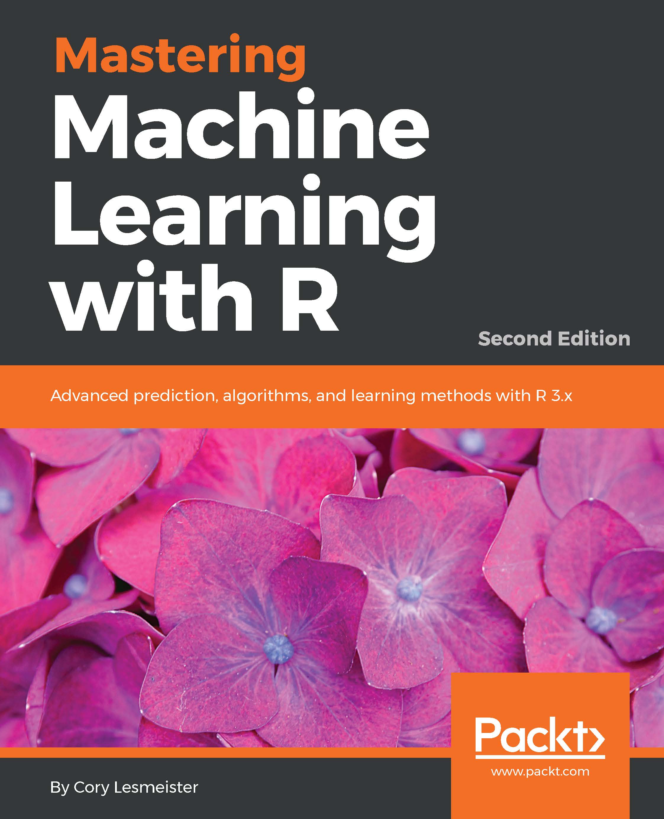
Mastering Machine Learning with R, Second Edition

You're reading from   Mastering Machine Learning with R, Second Edition Advanced prediction, algorithms, and learning methods with R 3.x

Arrow left icon
Product type Paperback
Published in Apr 2017
Publisher Packt
ISBN-13 9781787287471
Length 420 pages
Edition 2nd Edition
Languages
Arrow right icon
Author (1):
Arrow left icon
Cory Lesmeister Cory Lesmeister
Author Profile Icon Cory Lesmeister
Cory Lesmeister
Arrow right icon
View More author details
Toc

Table of Contents (17) Chapters Close

Preface 1. A Process for Success FREE CHAPTER 2. Linear Regression - The Blocking and Tackling of Machine Learning 3. Logistic Regression and Discriminant Analysis 4. Advanced Feature Selection in Linear Models 5. More Classification Techniques - K-Nearest Neighbors and Support Vector Machines 6. Classification and Regression Trees 7. Neural Networks and Deep Learning 8. Cluster Analysis 9. Principal Components Analysis 10. Market Basket Analysis, Recommendation Engines, and Sequential Analysis 11. Creating Ensembles and Multiclass Classification 12. Time Series and Causality 13. Text Mining 14. R on the Cloud 15. R Fundamentals 16. Sources

Regularization in a nutshell


You may recall that our linear model follows the form, Y = B0 + B1x1 +...Bnxn + e, and also that the best fit tries to minimize the RSS, which is the sum of the squared errors of the actual minus the estimate, or e12 + e22 + ... en2.

With regularization, we will apply what is known as shrinkage penalty in conjunction with the minimization RSS. This penalty consists of a lambda (symbol λ), along with the normalization of the beta coefficients and weights. How these weights are normalized differs in the techniques, and we will discuss them accordingly. Quite simply, in our model, we are minimizing (RSS + λ(normalized coefficients)). We will select λ, which is known as the tuning parameter, in our model building process. Please note that if lambda is equal to 0, then our model is equivalent to OLS, as it cancels out the normalization term.

So what does this do for us and why does it work? First of all, regularization methods are very computationally efficient. In...

lock icon The rest of the chapter is locked
Register for a free Packt account to unlock a world of extra content!
A free Packt account unlocks extra newsletters, articles, discounted offers, and much more. Start advancing your knowledge today.
Unlock this book and the full library FREE for 7 days
Get unlimited access to 7000+ expert-authored eBooks and videos courses covering every tech area you can think of
Renews at $19.99/month. Cancel anytime
Banner background image