Signal processing

Signal processing is the art of analyzing and manipulating signals arising in many fields of engineering. It deals with operations on or analysis of analog as well as digitized signals, representing time-varying or spatially varying physical quantities.

Julia has the functionality for processing signals built into the standard library along with a growing set of packages, and the speed of Julia makes it especially well suited to such analysis.

We can differentiate between 1D signals, such as audio signals, electrocardiogram (ECG) signals, variations in pressure and temperature, and so on, and 2D resulting in imagery from video and satellite data streams. In this section, I will mainly focus on the former, but the techniques carry over in a straightforward fashion to the 2D cases.

Frequency analysis

A signal is simply a measurable quantity that varies in time and/or space. The key insight of signal processing is that a signal in time can be represented by a linear combination of sinusoids at different frequencies.

There exists an operation called the Fourier transform (FT), which takes an x(t) function of time that is called the time-domain signal and computes the weights of its sinusoidal components. These weights are represented as an X(f) function of frequency called the frequency-domain signal.

The FT takes a continuous function and produces another continuous function as a function of the frequencies of which it is composed. In digital signal processing, since we operate on signals in discrete time, we use the discrete FT (DFT).

This takes a set of N samples in time and produces weights at N different frequencies. Julia’s signal processing library, as with most common signal processing software packages, computes DFTs by using a class of algorithms known as fast FTs (FFTs).

Smoothing and filtering

First, we will generate a signal from three sinusoids and visualize it:

julia> using Plots, FFTW
julia> fq = 500.0;
julia> N = 512;
julia> T = 6 / fq;
julia> t = collect(range(0, stop=T, length=N));
julia> x1 = sin.(2π * fq * t);
julia> x2 = cos.(8π * fq * t);
julia> x3 = cos.(16π * fq * t);
julia> x = x1 + 0.4*x2 + 0.2*x3;

Now, use the rfft function (the real FFT function) since our input signal is composed entirely of real numbers, as opposed to complex numbers. This allows us to optimize by only computing the weights for frequencies from 1 to N/2+1.

The higher frequencies are simply a mirror image of the lower ones, so they do not contain any extra information. We will need to use the absolute magnitude (modulus) of the output of rfft() because the outputs are complex numbers. Right now, we only care about the magnitude and not the phase of the frequency domain signal:

julia> X = rfft(x);
julia> sr = N / T;
julia> fd = LinRange(0, sr/2, Int(N/2) + 1)
julia> plot(fd, abs(X)[1:N/8])

This transforms the time domain representation of the signal (amplitude versus time) into one in the frequency domain (magnitude versus frequency).

The following figure shows the two representations:

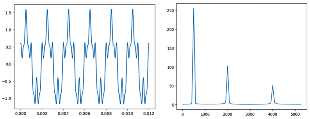
Figure 7.1 – FFT of a sinusoidal function

Now, we can add some high-frequency noise to the signal:

julia> ns = 0.1*randn(length(x));
julia> xn = x + ns;

Then, use a convolution procedure in the time domain to attempt to remove it. In essence, this is a moving average (MA) smoothing technique.

We define a 16-element window and use a uniform distribution, although it might be sensible to use a Gaussian or parabolic one that would weigh the nearest neighbors more appropriately:

julia> M = 16;
julia> xm = ones(Float64, M) / M;

We then apply a convolution function in the DSP package to xm and xn:

julia> using DSP
julia> xf = conv(xn, xm);
julia> t = [0:length(xf) - 1] / sr

It is important that the sum of the weights is 1.

The following figure shows the noisy signal together with the filtered one:

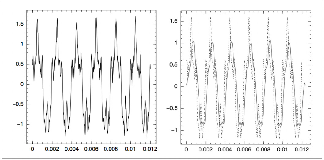
Figure 7.2 – Comparison of noisy and filtered signals of the sinusoid

The main carrier wave is recovered and the noise is eliminated, but given the size of the window chosen, the convolution has a drastic effect on the higher-frequency components.

Digital signal filters

MA filters (convolution) work well for removing noise if the frequency of the noise is much higher than the principal components of a signal.

A common requirement in RF communications is to retain parts of the signal but to filter out the others. The simplest filter of this sort is a low-pass filter. This is a filter that allows sinusoids below a critical frequency to go through unchanged while attenuating signals above the critical frequency. Clearly, this is a case where the processing is done in the frequency domain.

Filters can also be constructed to retain sinusoids above the critical frequency (high pass), or within a specific frequency range (medium band). Julia provides a set of signal processing packages as the DSP.jl group (https://github.com/JuliaDSP/DSP.jl), and we will apply some of the routines to filter out noise on the signal we created in the previous section:

julia> using DSP
julia> responsetype = Lowpass(0.2);
julia> prototype = Elliptic(4, 0.5, 30);
julia> tf = convert(PolynomialRatio,
                digitalfilter(responsetype prototype))
julia> numerator_coefs = coefb(tf);
julia> denominator_coefs = coefa(tf);

This constructs a fourth-order elliptic low-pass filter with normalized cut-off frequency 0.2, 0.5 dB of passband ripple, and 30 dB attenuation in the stopband.

Then, the coefficients of the numerator and denominator of the transfer function will be this:

julia> responsetype = Bandpass(10, 40; fs=1000);
julia> prototype = Butterworth(4);
julia> xb = filt(digitalfilter(responsetype,prototype),x);
julia> plot(xb)

This code filters the data in the x signal, sampled at 1,000 Hz, with a fourth-order Butterworth bandpass filter between 10 and 40 Hz.

The resultant signal is displayed as follows:

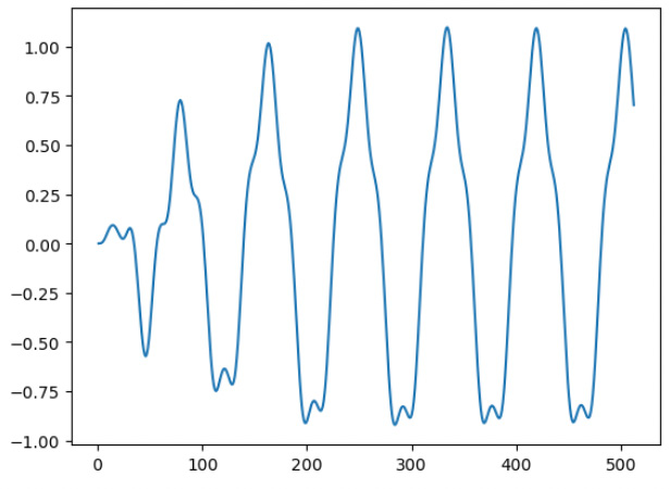
Figure 7.3 – Application of a Butterworth bandpass filter

While being cleaner than convolution, this still affects high frequencies.

Also, while the bandpass filter is infinite in its extent, the one constructed is truncated, and this means that the initial portion of the signal is modulated.

Image convolutions

Frequency-based methods can be applied to 2D signals, such as those from video and satellite data streams. High-frequency noise in imagery is termed “speckle.” Essentially, due to the orthogonality of the FFT, processing involves applying a series of row-wise and column-wise FFTs independently of each other.

The DSP package has routines to deal with both 1D and 2D cases. Also, the convolution techniques we looked at in the Frequency analysis section are often employed in enhancing or transforming images, and we will finish by looking at a simple example using a 3x3 convolution kernel.

The kernel needs to be zero-summed; otherwise, the histogram range of the image is altered. We will look at the Lena image that is provided as a 512x512 PGM image:

julia> cd(ENV["HOME"]*"/MJ2/DataSources");
julia> img = open(Files/lena.pgm");
julia> magic = chomp(readline(img));
julia> params = chomp(readline(img));
julia> pm = split(params)
# Remember the GSD
julia> try
  global wd = parse(Int64,pm[1]);
  global ht = parse(Int64,pm[2]);
catch
  error("Can't figure out the image dimensions")
end
# Version 1.0 way of defining a byte array
# readbytes!() will read in place
julia> data = Array{UInt8,2}(undef,wd,ht)
julia> readbytes!(img, data, wd*ht);
julia> data = reshape(data,wd,ht);
julia> close(img);

The preceding code reads the PGM image and stores the imagery as a byte array in data, reshaping it to be wd by ht.

Now, we define the two 3x3 Gx and Gy kernels:

julia> Gx = [1 2 1; 0 0 0; -1 -2 -1];
julia> Gy = [1 0 -1; 2 0 -2; 1 0 -1];

The following loops over blocks of the original image applying Gx and Gy, constructs the modulus of each convolution, and outputs the transformed image as dout, again as a PGM image. We need to be a little careful that the imagery is still preserved as a byte array:

julia> dout = copy(data);
julia> for i = 2:wd-1
  for j = 2:ht-1
    temp = data[i-1:i+1, j-1:j+1];
    x = sum(Gx.*temp)
    y = sum(Gy.*temp)
    p = Int64(floor(sqrt(x*x + y*y)))
    dout[i,j] = (p < 256) ? UInt8(p) : 0xff
    end
end
# ... and output the result
julia> DS = ENV["HOME"]*"/MJ2/DataSources"
julia> out = open("$DS/Files/lenaX.pgm","w");
julia> println(out,magic);
julia> println(out,params);
julia> write(out,dout);
julia> close(out);

We can display the convoluted image using the ImageView package we used previously to view the Julia set:

julia> using Images. ImageView
julia> img = load("$DS/Files/lenaX.pgm")
julia> imshow(img)

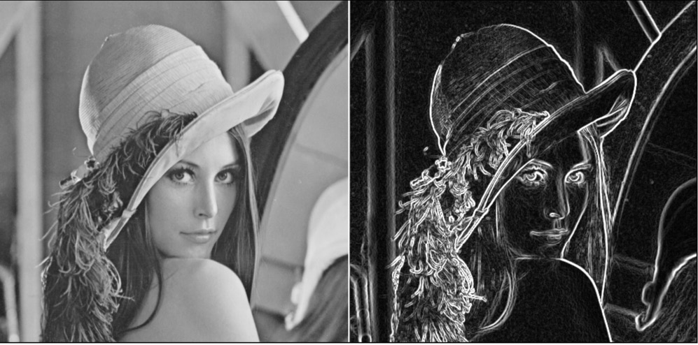
Figure 7.4 – Original and convoluted images of “Lena”

We will leave the discussion of imagery but will be returning to it for a more extensive look in the final section of the next chapter. Now, I will switch to the topic of the solution of DEs