Search icon CANCEL
Subscription
0
Cart icon
Your Cart (0 item)
Close icon
You have no products in your basket yet
Save more on your purchases! discount-offer-chevron-icon
Savings automatically calculated. No voucher code required.
Arrow left icon
Explore Products
Best Sellers
New Releases
Books
Videos
Audiobooks
Learning Hub
Free Learning
Arrow right icon
Arrow up icon
GO TO TOP
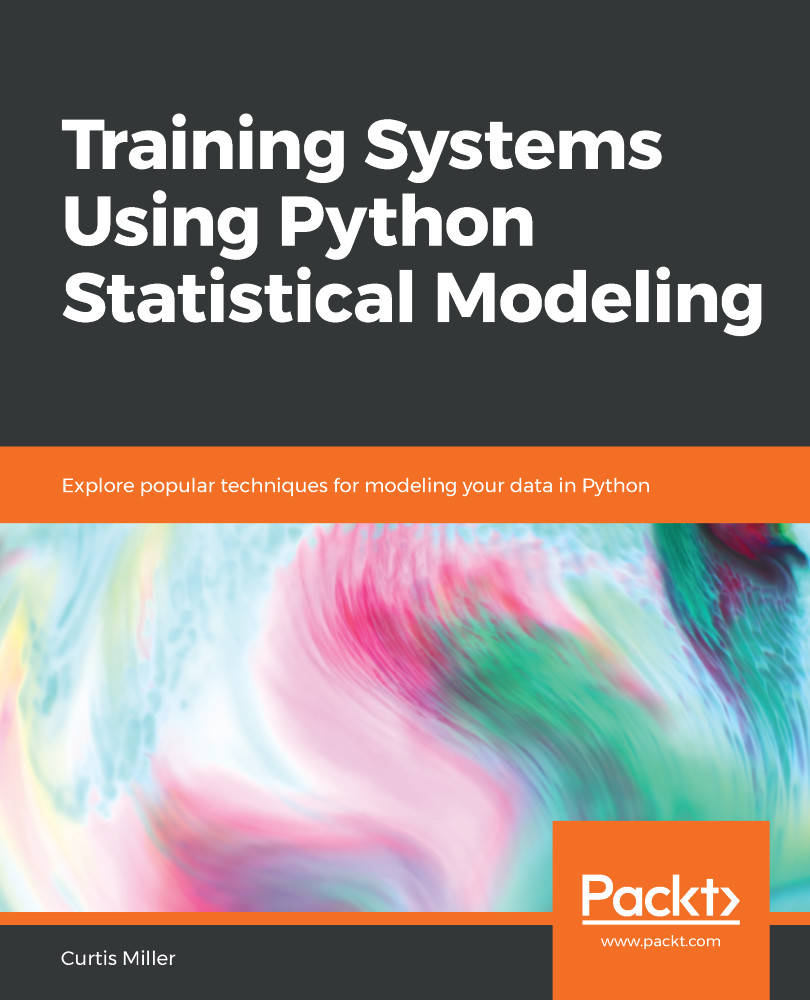
Training Systems Using Python Statistical Modeling

You're reading from   Training Systems Using Python Statistical Modeling Explore popular techniques for modeling your data in Python

Arrow left icon
Product type Paperback
Published in May 2019
Publisher Packt
ISBN-13 9781838823733
Length 290 pages
Edition 1st Edition
Languages
Tools
Arrow right icon
Author (1):
Arrow left icon
Curtis Miller Curtis Miller
Author Profile Icon Curtis Miller
Curtis Miller
Arrow right icon
View More author details
Toc

Computing descriptive statistics

In this section, we will review methods for obtaining descriptive statistics from data that is stored in a pandas DataFrame. We will use the pandas library to compute statistics from the data. So, let's jump right in!

DataFrames come equipped with many methods for computing common descriptive statistics for the data they contain. This is one of the advantages of storing data in DataFrames—working with data stored this way is easy. Getting common descriptive statistics, such as the mean, the median, the standard deviation, and more, is easy for data that is present in DataFrames. There are methods that can be called in order to quickly compute each of these. We will review several of these methods now.

If you want a basic set of descriptive statistics, just to get a sense of the contents of the DataFrame, consider using the describe() method. It includes the mean, standard deviation, an account of how much data there is, and the five-number summary built in.

Sometimes, the statistic that you want isn't a built-in DataFrame method. In this case, you will write a function that works for a pandas series, and then apply that function to each column using the apply() method.

Preprocessing the data

Now let's open up the Jupyter Notebook and get started on our first program, using the methods that we discussed in the previous section:

  1. The first thing we need to do is load the various libraries that we need. We will also load the iris dataset from the scikit-learn library, using the following code:

  1. After importing all the required libraries and the dataset, we will go ahead and create an object called iris_obj, which loads the iris dataset into an object. Then, we will go ahead and use the data method to preview the dataset; and this results in the following output:

Notice that it's a NumPy array. This contains a lot of the data that we want, and each of these columns corresponds to a feature.

  1. We will now see what those feature names are in the following output:

As you can see here, the first column shows the sepal length, the next column shows the sepal width, the third column shows the petal length, and the final column shows the petal width.

  1. Now, there is a fifth column that is not displayed hereit's referred to as the target column. This is stored in a separate array; we will now look at this column as follows:

This displays the target column in an array.

  1. Now, if you want to see the labels of the array header, we can use the following code:

As you can see, the target column consists of data with three different labels. The flowers come from either the setosa, the versicolor, or the virginica species.

  1. Our next step is to take this dataset and turn it into a pandas DataFrame, using the following code:

This results in the following output:

As you can see, we have successfully loaded the data into a DataFrame.

  1. We can see that the species column still shows the various species using numeric values. So, we will replace the final column, which indicates the various species, with strings that indicate the values, rather than numbers, using the following code block:

The following screenshot shows the result:

As you can see, the species column now has the actual species namesthis makes it much easier to work with the data.

Now, for this dataset, the fact that each flower comes from a different species suggests that we may want to actually group the data when we're doing statistical summariestherefore, we can try grouping by species.

  1. So, we will now group the dataset values using the species column as the anchor, and then print out the details of each group to make sure that everything is working. We will use the following lines of code to do so:

This results in the following output:

Now that the data has been loaded and set up, we will use it to perform some basic statistical operations in the next section.

Computing basic statistics

Now we can use the DataFrame that we created to get some basic numbers; we will use the following steps to do so:

  1. We can count how much data there is through the count() method, as shown in the following screenshot:

We can see that there are 150 observations. Note that this excludes NA values (that is, missing values), so it is possible that not all of these observations will be 150.

  1. We can also compute the sample mean, which is the arithmetic average of all the numbers in the dataset, by simply calling the mean() method, as shown in the following screenshot:

Here, we can see the arithmetic means for the numeric columns. The sample mean can also be calculated arithmetically, using the following formula:

  1. Next, we can compute the sample median using the median() method:

Here, we can see the median values; the sample median is the middle data point, which we get after ordering the dataset. It can be computed arithmetically by using the following formula:

Here, x(n) represents ordered data.

  1. We can compute the variance as follows:

The sample variance is a measure of dispersion and is roughly the average squared distance of a data point from the mean. It can be calculated arithmetically, as follows:

  1. The most interesting quantity is the sample standard deviation, which is the square root of the variance. It is computed as follows:

The standard deviation is the square root of the variance and is interpreted as the average distance that a data point is from the mean. It can be represented arithmetically, as follows:

  1. We can also compute percentiles; we do that by defining the value of the percentile that you want to see using the following command:
iris.quantile(.p)

So, here, roughly p% of the data is less than that percentile.

  1. Let's find out the 1st, 3rd, 10th, and 95th percentiles as an example, as follows:
  1. Now, we will compute the interquartile range (IQR) between the 3rd and 1st quantile using the following function:
  1. Other interesting quantities include the maximum value of the dataset, and the minimum value of the dataset. Both of these values can be computed as follows:

Most of the methods mentioned here also work with grouped data. As an exercise, try summarizing the data that we grouped in the previous section, using the previous methods.

  1. Another useful method includes the describe() method. This method can be useful if all you want is just a basic statistical summary of the dataset:

Note that this method includes the count, mean, standard deviations, the five-number summaryfrom the minimum to the maximum, and the quantiles in between. This will also work for grouped data. As an exercise, why don't you try finding the summary of the grouped data?

  1. Now, if we want a custom numerical summary, then we can write a function that will work for a pandas series, and then apply that to the columns of a DataFrame. For example, there isn't a function that computes the range of a dataset, which is the difference between the maximum and the minimum of the dataset. So, we will define a function that can compute the range if it were given a pandas series; here, you can see that by sending it to apply(), you get the ranges that you want:

Notice that I was more selective in choosing columns in terms of which columns to work with. Previously, a lot of the methods were able to weed out columns that weren't numeric; however, to use apply(), you need to specifically select the columns that are numeric, otherwise, you may end up with an error.

  1. We can't directly use the preceding code if we want to filter for grouped data. Instead, we can use the .aggregate() method, as follows:

Thus, we have learned all about computing various statistics using the methods present in pandas. In the next section, we will look at classical statistical inference, specifically with inference for a population proportion.

You have been reading a chapter from
Training Systems Using Python Statistical Modeling
Published in: May 2019
Publisher: Packt
ISBN-13: 9781838823733
Register for a free Packt account to unlock a world of extra content!
A free Packt account unlocks extra newsletters, articles, discounted offers, and much more. Start advancing your knowledge today.
Unlock this book and the full library FREE for 7 days
Get unlimited access to 7000+ expert-authored eBooks and videos courses covering every tech area you can think of
Renews at $19.99/month. Cancel anytime
Banner background image