Graphics and standard plots
The graphics package was originally developed based on the experience of the graphics environment in R. The approach implemented in this package is based on the principle of the pen-on-paper model, where the plot is drawn in the first function call and once content is added, it cannot be deleted or modified.
In general, the functions available in this package can be divided into high-level and low-level functions. High-level functions are functions capable of drawing the actual plot, while low-level functions are functions used to add content to a graph that was already created with a high-level function.
Tip
Downloading the example code
You can download the example code files from your account at http://www.packtpub.com for all the Packt Publishing books you have purchased. If you purchased this book elsewhere, you can visit http://www.packtpub.com/support and register to have the files e-mailed directly to you.
Let's assume that we would like to have a look at how age is related to the circumference of the trees in our dataset Orange; we could simply plot the data on a scatter plot using the high-level function plot() as shown in the following code:
plot(age~circumference, data=Orange)
This code creates the graph in Figure 1.3. As you would have noticed, we obtained the graph directly with a call to a function that contains the variables to plot in the form of y~x, and the dataset to locate them. As an alternative, instead of using a formula expression, you can use a direct reference to x and y, using code in the form of plot(x,y). In this case, you will have to use a direct reference to the data instead of using the data argument of the function. Type in the following code:
plot(Orange$circumference, Orange$age)
The preceding code results in the following output:

Figure 1.3: Simple scatterplot of the dataset Orange using graphics
For the time being, we are not interested in the plot's details, such as the title or the axis, but we will simply focus on how to add elements to the plot we just created. For instance, if we want to include a regression line as well as a smooth line to have an idea of the relation between the data, we should use a low-level function to add the just-created additional lines to the plot; this is done with the lines() function:
plot(age~circumference, data=Orange)   ###Create basic plot
abline(lm(Orange$age~Orange$circumference), col="blue")
lines(loess.smooth(Orange$circumference,Orange$age), col="red")
The graph generated as the output of this code is shown in Figure 1.4:

Figure 1.4: This is a scatterplot of the Orange data with a regression line (in blue) and a smooth line (in red) realized with graphics
As illustrated, with this package, we have built a graph by first calling one function, which draws the main plot frame, and then additional elements were included using other functions. With graphics, only additional elements can be included in the graph without changing the overall plot frame defined by the plot() function. This ability to add several graphical elements together to create a complex plot is one of the fundamental elements of R, and you will notice how all the different graphical packages rely on this principle. If you are interested in getting other code examples of plots in graphics, there is also some demo code available in R for this package, and it can be visualized with demo(graphics).
In the coming sections, you will find a quick reference to how you can generate a similar plot using graphics and ggplot2. As will be described in more detail later on, in ggplot2, there are two main functions to realize plots, ggplot() and qplot(). The function qplot() is a wrapper function that is designed to easily create basic plots with ggplot2, and it has a similar code to the plot() function of graphics. Due to its simplicity, this function is the easiest way to start working with ggplot2, so we will use this function in the examples in the following sections. The code in these sections also uses our example dataset Orange; in this way, you can run the code directly on your console and see the resulting output.
Scatterplots with individual data points
To generate the plot generated using graphics, use the following code:
plot(age~circumference, data=Orange)
The preceding code results in the following output:

To generate the plot using ggplot2, use the following code:
qplot(circumference,age, data=Orange)
The preceding code results in the following output:

Scatterplots with the line of one tree
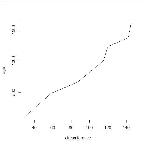
To generate the plot using graphics, use the following code:
plot(age~circumference, data=Orange[Orange$Tree==1,], type="l")
The preceding code results in the following output:
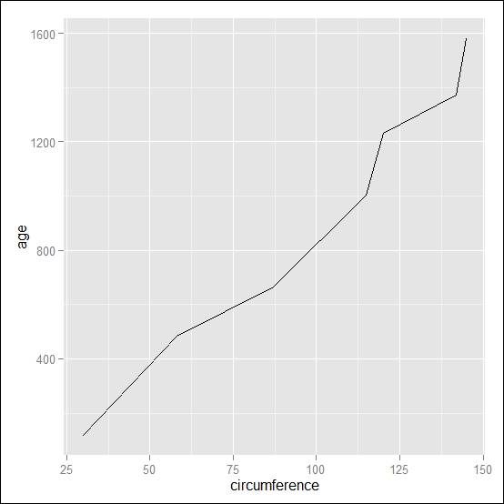
To generate the plot using ggplot2, use the following code:
qplot(circumference,age, data=Orange[Orange$Tree==1,], geom="line")
The preceding code results in the following output:
Scatterplots with the line and points of one tree
To generate the plot using graphics, use the following code:
plot(age~circumference, data=Orange[Orange$Tree==1,], type="b")
The preceding code results in the following output:

To generate the plot using ggplot2, use the following code:
qplot(circumference,age, data=Orange[Orange$Tree==1,], geom=c("line","point"))
The preceding code results in the following output:

Boxplots of the orange dataset
To generate the plot using graphics, use the following code:
boxplot(circumference~Tree, data=Orange)
The preceding code results in the following output:

To generate the plot using ggplot2, use the following code:
qplot(Tree,circumference, data=Orange, geom="boxplot")
The preceding code results in the following output:

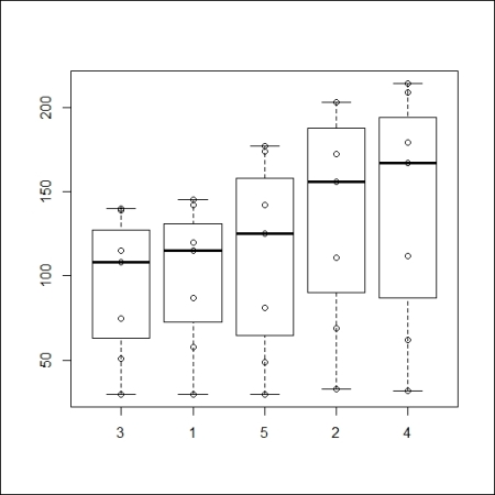
Boxplots with individual observations
To generate the plot using graphics, use the following code:
boxplot(circumference~Tree, data=Orange)
points(circumference~Tree, data=Orange)
The preceding code results in the following output:
To generate the plot using ggplot2, use the following code:
qplot(Tree,circumference, data=Orange, geom=c("boxplot","point"))
The preceding code results in the following output:

Histograms of the orange dataset
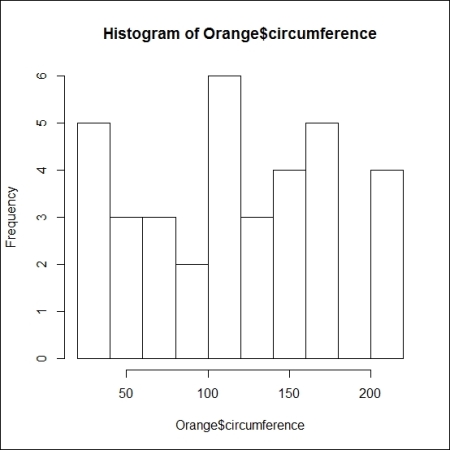
To generate the plot using graphics, use the following code:
hist(Orange$circumference)
The preceding code results in the following output:
To generate the plot using ggplot2, use the following code:
qplot(circumference, data=Orange, geom="histogram")
The preceding code results in the following output:

Histograms with the reference line at the median value in red
To generate the plot using graphics, use the following code:
hist(Orange$circumference)
abline(v=median(Orange$circumference), col="red")
The preceding code results in the following output:

To generate the plot using ggplot2, use the following code:
qplot(circumference, data=Orange, geom="histogram")+geom_vline(xintercept = median(Orange$circumference), colour="red")
The preceding code results in the following output:


