Understanding mean, median, and mode

Mean, median, and mode describe the central tendency in some way. Mean and median are only applicable to numerical variables whereas mode is applicable to both categorical and numerical variables. In this section, we will be focusing on mean, median, and mode for numerical variables as their numerical interactions usually convey interesting observations.

Mean

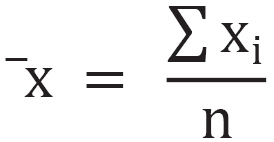
Mean, or arithmetical mean, measures the weighted center of a variable. Let's use n to denote the total number of entries and as the index. The mean reads as follows:

Mean is influenced by the value of every entry in the population.

Let me give an example. In the following code, I will generate 1,000 random numbers from 0 to 1 uniformly, plot them, and calculate their mean:

import random
random.seed(2019)
plt.figure(figsize=(8,6))
rvs = [random.random() for _ in range(1000)]
plt.hist(rvs, bins=50)
plt.title("Histogram of Uniformly Distributed RV");

The resulting histogram plot appears as follows:

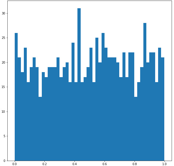
Figure 2.4 – Histogram distribution of uniformly distributed variables between 0 and 1

The mean is around 0.505477, pretty close to what we surmised.

Median

Median measures the unweighted center of a variable. If there is an odd number of entries, the median takes the value of the central one. If there is an even number of entries, the median takes the value of the mean of the central two entries. Median may not be influenced by every entry's value. On account of this property, median is more robust or representative than the mean value. I will use the same set of entries as in previous sections as an example.

The following code calculates the median:

np.median(rvs)

The result is 0.5136755026003803. Now, I will be changing one entry to 1,000, which is 1,000 times larger than the maximal possible value in the dataset and repeat the calculation:

rvs[-1]=1000
print(np.mean(rvs))
print(np.median(rvs))

The results are 1.5054701085937803 and 0.5150437661964872. The mean increased by roughly 1, but the median is robust.

The relationship between mean and median is usually interesting and worth investigating. Usually, the combination of a larger median and smaller mean indicates that there are more points on the bigger value side, but that an extremely small value also exists. The reverse is true when the median is smaller than the mean. We will demonstrate this with some examples later.

Mode

The mode of a set of values is the most frequent element in a set. It is evident in a histogram plot such that it represents the peak(s). If the distribution has only one mode, we call it unimodal. Distributions with two peaks that don't have to have equal heights are referred to as bimodal.

Bimodals and bimodal distribution

Sometimes, the definition of bimodal is corrupted. The property of being bimodal usually refers to the property of having two modes, which, according to the definition of mode, requires the same height of peaks. However, the term bimodal distribution often refers to a distribution with two local maxima. Double-check your distribution and state the modes clearly.

The following code snippet demonstrates two distributions with unimodal and bimodal shapes, respectively:

r1 = [random.normalvariate(0.5,0.2) for _ in range(10000)]
r2 = [random.normalvariate(0.2,0.1) for _ in range(5000)]
r3 = [random.normalvariate(0.8,0.2) for _ in range(5000)]
fig, axes = plt.subplots(1,2,figsize=(12,5))
axes[0].hist(r1,bins=100)
axes[0].set_title("Unimodal")
axes[1].hist(r2+r3,bins=100)
axes[1].set_title("Bimodal");

The resulting two subplots appear as follows:

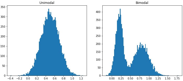
Figure 2.5 – Histogram of unimodal and bimodal datasets with one mode and two modes

So far, we have talked about mean, median and mode, mean, median and mode, which are the first three statistics of a dataset. They are the start of almost all exploratory data analysis.