Introducing the robot and our development environment
This is a book about robots and AI, so we really need to have a robot to use for all of our practical examples. As we will discuss in Chapter 2 at some length, I have selected robot hardware and software that will be accessible to the average reader. The particular brand and type are not important, and I’ve upgraded Albert considerably since the first edition was published some five years ago. In the interest of keeping things up to date, we are putting all of the hardware details in the GitHub repository for this book.
As shown in the following photographs taken from two different perspectives, my robot has new omnidirectional wheels, a mechanical six-degree-of-freedom arm, and a computer brain:
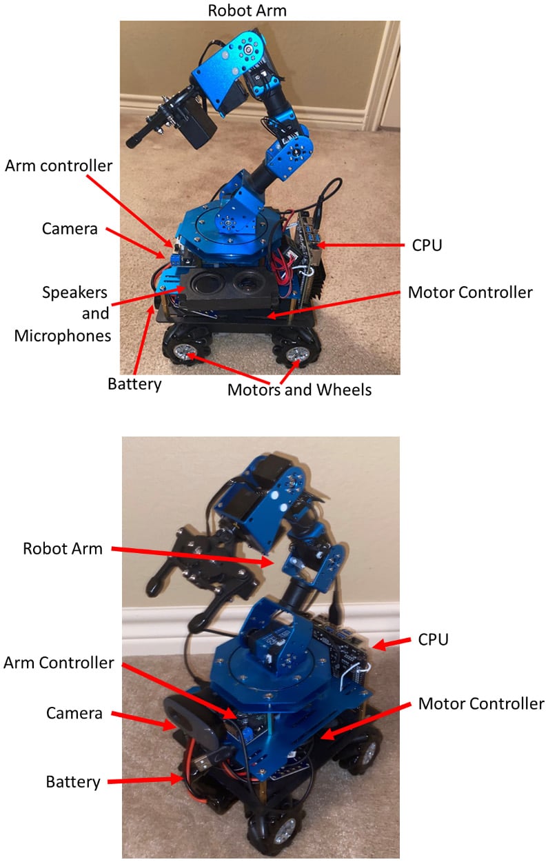
Figure 1.2 – Albert the robot has wheels and a mechanical arm
I’ll call it Albert, since it needs some sort of name, and I like the reference to Prince Albert, consort of Queen Victoria, who was famous for taking marvelous care of their nine children. All nine of his children survived to adulthood, which was a rarity in the Victorian age, and he had 42 grandchildren. He went by his middle name; his actual first name was Francis.
Our tasks in this book center around picking up toys in an interior space, so our robot has a solid base with four motors and omni wheels for driving over carpet. Our steering method is the tank type, or differential drive, where we steer by sending different commands to the wheel motors. If we want to go straight ahead, we set all four motors to the same forward speed. If we want to travel backward, we reverse both motors the same amount. Turns are accomplished by moving one side forward and the other backward (which makes the robot turn in place) or by giving one side more forward drive than the other. We can make any sort of turn this way. The omni wheels allow us to do some other tricks as well – we can turn the wheels toward each other and translate directly sideways, and even turn in a circle while pointing at the same spot on the ground. We will mostly drive like a truck or car but will use the y-axis motion occasionally to line things up. Speaking of axes, I’ll use the x axis to mean that the robot will move straight ahead, the y axis refers to horizontal movement from side to side, and the z axis is up and down, which we need for the robot’s arm.
In order to pick up toys, we need some sort of manipulator, so I’ve included a six-axis robot arm that imitates a shoulder–elbow–wrist–hand combination that is quite dexterous and, since it is made out of standard digital servos, quite easy to wire and program.
The main control of the Albert robot is the Nvidia Nano single-board computer (SBC), which talks to the operator via a USB Wi-Fi dongle. The Nvidia talks to an Arduino Mega 2560 microcontroller and motor controller that we will use to control motors via Pulse Width Modulation (PWM) pulses. The following figure depicts the internal components of the robot:
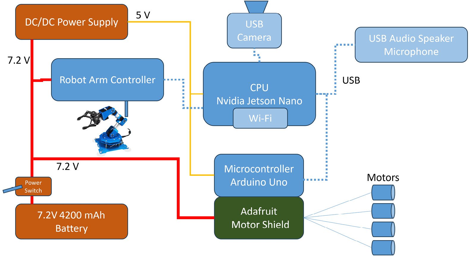
Figure 1.3 – Block diagram of the robot
We will be primarily concerned with the Nvidia Nano SBC, which is the brains of our robot. We will set up the rest of the components once and not change them for the entire book.
The Nvidia Nano acts as the main interface between our control station, which is a PC running Windows, and the robot itself via a Wi-Fi network. Just about any low-power, Linux-based SBC can perform this job, such as a BeagleBone Black, Odroid XU4, or an Intel Edison. One of the advantages of the Nano is that it can use its Graphics Processing Units (GPUs) to speed up the processing of neural networks.
Connected to the SBC is an Arduino with a motor controller. The Nano talks through a USB port addressed as a serial port. We also need a 5V regulator to provide the proper power from the 11.1V rechargeable lithium battery power pack into the robot. My power pack is a rechargeable 3S1P (three cells in series and one in parallel) 2700 Ah battery (normally used for quadcopter drones) and came with the appropriate charger. As with any lithium battery, follow all of the directions that come with the battery pack and recharge it in a metal box or container in case of fire.
Software components (ROS, Python, and Linux)
I am going to direct you once again to the Git repository to see all of the software that runs the robot, but I’ll cover the basics here to remind you. The base operating system for the robot is Linux running on an Nvidia Nano SBC, as we said. We are using the ROS 2 to connect all of our various software components together, and it also does a wonderful job of taking care of all of the finicky networking tasks such as setting up sockets and establishing connections. It also comes with a great library of already prepared functions that we can just take advantage of, such as a joystick interface. ROS 2 is not a true operating system that controls the whole computer like Linux or Windows does, but rather is a backbone of communications and interface standards and utilities that make putting together a robot a lot simpler. The name I like to use for this type of system is Modular Open System Architecture (MOSA). ROS 2 uses a publish/subscribe technique to move data from one place to another that truly decouples the programs that produce data (such as sensors and cameras) from those programs that use data, such as controls and displays. We’ll be making a lot of our own stuff and only using a few ROS functions. Packt has several great books for learning ROS; my favorite is Effective Robotics Programming with ROS.
The programming language we will use throughout this book, with a couple of minor exceptions, will be Python. Python is a great language for this purpose for two great reasons: it is widely used in the robotics community in conjunction with ROS, and it is also widely accepted in the machine learning and AI community. This double whammy makes using Python irresistible. Python is an interpreted language, which has three amazing advantages for us:
- Portability: Python is very portable between Windows, Mac, and Linux. Usually, you can get by with just a line or two of changes if you use a function out of the operating system, such as opening a file. Python has access to a huge collection of C/C++ libraries that also add to its utility.
- No compilation: As an interpreted language, Python does not require a compile step. Some of the programs we are developing in this book are pretty involved, and if we wrote them in C or C++, it would take 10 or 20 minutes of build time each time we made a change. You can do a lot with that much time, which you can spend getting your program to run and not waiting for the make process to finish.
- Isolation: This is a benefit that does not get talked about much but having had a lot of experience with crashing operating systems with robots, I can tell you that the fact that Python’s interpreter is isolated from the core operating system means that having one of your Python ROS programs crash the computer is very rare. A computer crash means rebooting the computer and also probably losing all of the data you need to diagnose the crash. I had a professional robot project that we moved from Python to C++, and immediately the operating system crashes began, which shot the reliability of our robot. If a Python program crashes, another program can monitor that and restart it. If the operating system has crashed, there is not much you can do without some extra hardware that can push the Reset button for you.
Before we dive into the coding of our base control system, let’s talk about the theory we will use to create a robust, modular, and flexible control system for robotics.
Robot control systems and a decision-making framework
As I mentioned earlier in this chapter, we are going to use two sets of tools in the sections: soft real-time control and the OODA loop. One gives us a base for controlling the robot easily and consistently, and the other provides a basis for the robot’s autonomy.
How to control your robot
The basic concept of how a robot works, especially one that drives, is simple. There is a master control loop that does the same thing over and over – reads data from the sensors and motor controller, looks for commands from the operator (or the robot’s autonomy functions), makes any changes to the state of the robot based on those commands, and then sends instructions to the motors or effectors to make the robot move.
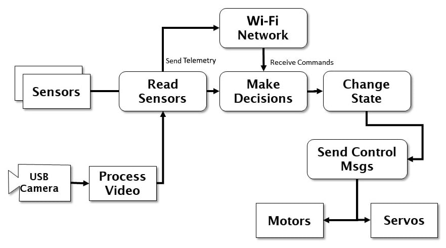
Figure 1.4 – Robot control loop
The preceding diagram illustrates how we have instantiated the OODA loop in the software and hardware of our robot. The robot can either act autonomously or accept commands from a control station connected via a wireless network.
What we need to do is perform this control loop in a consistent manner all of the time. We need to set a base frame rate or basic update frequency that sets the timing of our control loop. This makes all the systems of the robot perform together. Without some sort of time manager, each control cycle of the robot takes a different amount of time to complete, and any sort of path planning, position estimate, or arm movement becomes very complicated. ROS does not provide a time manager as it is inherently non-synchronous; if required, we have to create one ourselves.
Using control loops
In order to have control of our robot, we have to establish some sort of control or feedback loop. Let’s say that we tell the robot to move 12 inches (30 cm) forward. The robot must send a command to the motors to start moving forward, and then have some sort of mechanism to measure 12 inches of travel. We can use several means, but let’s just use a clock. The robot moves 3 inches (7.5 cm) per second. We need the control loop to start the movement, and then each update cycle, or time through the loop, check the time and see whether four seconds have elapsed. If they have, then it sends a stop command to the motors. The timer is the control, four seconds is the set point, and the motor is the system that is controlled. The process also generates an error signal that tells us what control to apply (in this case, to stop). Let’s look at a simple control loop:
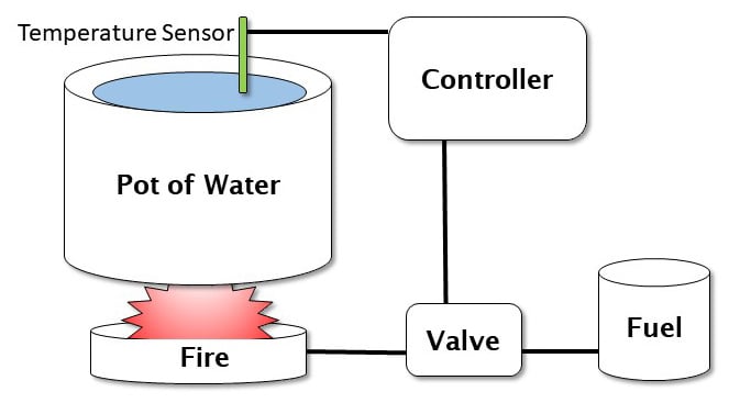
Figure 1.5 – Sample control loop – maintaining the temperature of a pot of water
Based on the preceding figure, what we want is a constant temperature in the pot of water. The valve controls the heat produced by the fire, which warms the pot of water. The temperature sensor detects whether the water is too cold, too hot, or just right. The controller uses this information to control the valve for more heat. This type of schema is called a closed loop control system.
You can think of this also in terms of a process. We start the process, and then get feedback to show our progress so that we know when to stop or modify the process. We could be doing speed control, where we need the robot to move at a specific speed, or pointing control, where the robot aims or turns in a specific direction.
Let’s look at another example. We have a robot with a self-charging docking station, with a set of light-emitting diodes (LEDs) on the top as an optical target. We want the robot to drive straight into the docking station. We use the camera to see the target LEDs on the docking station. The camera generates an error signal, which is used to guide the robot toward the LEDs. The distance between the LEDs also gives us a rough range to the dock. This process is illustrated in the following figure:
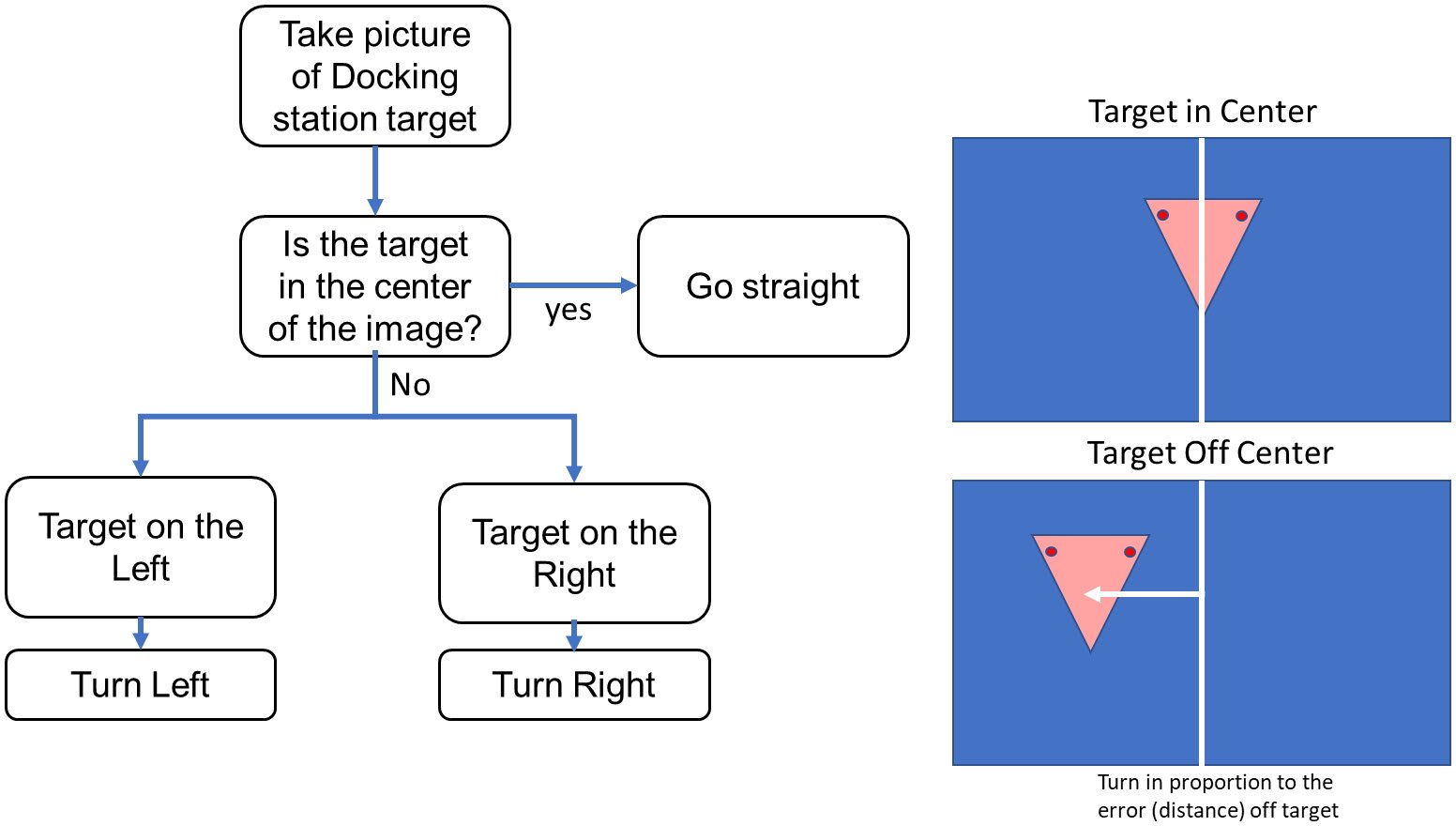
Figure 1.6 – Target tracking for a self-docking charging station
Let’s understand this in some more detail:
- Let’s say that the LEDs in the figure are off to the left of the center 50% and the distance from the robot to the target is 3 feet (1 m). We send that information through a control loop to the motors – turn left a bit and drive forward a bit.
- We then check again, and the LEDs are closer to the center (40%) and the distance to the target is 2.9 feet or 90 cm. Our error signal is a bit less, and the distance is a bit less. We’ll have to develop a scaling factor to determine how many pixels equate to how much turn rate, which is measured as a percentage of full power. Since we are using a fixed camera and lens, this will be a constant.
- Now we send a slower turn and a slower movement to the motors this update cycle. We end up exactly in the center and come to zero speed just as we touch the docking station.
For those people currently saying, “But if you use a PID controller …”, yes, you are correct – you also know that I’ve just described a P or proportional control scheme. We can add more bells and whistles to help prevent the robot from overshooting or undershooting the target due to its own weight and inertia and to damp out oscillations caused by those overshoots.
A PID controller is a type of control system that uses three types of inputs to manage a closed-loop control system. A proportional control uses a multiple of the detected error to drive a control.
For example, in our pot of water, we measure the error in the temperature. If the desired temperature is 100°C and we measure 90°C with our thermometer, then the error in the temperature is 10 °C. We need to add more heat by opening the valve in proportion to the temperature error. If the error is 0, the change in the value is 0. Let’s say that we try changing the value of the valve by 10% for a 10°C error. So we multiply 10°C by 0.01 to set our valve position to +0.1. This 0.01 value is our P term or proportional constant.
In our next sample, we see that the temperature of our pot is now 93°C and our error is 7°C. We change our valve position to +0.07, slightly less than before. We will probably find that by using this method, we will overshoot the desired temperature due to the hysteresis of the water – it takes a while for the water to heat up, creating a delay in the response. We will end up overheating the water and overshooting our desired temperature. One way to help prevent that is with the D term of the PID controller, that is, a derivative term. You remember that a derivative describes the slope of the line of a function – in this case, the temperature curve we measure. The y axis of our temperature graph is time, so we have delta temperature/delta time. To add a D term to our controller, we also add in the difference between the error of the last sample and the error of this sample (-10 – (-7) = -3). We add this to our control by multiplying this value times a constant, D. The integral term is just the cumulative sum of the error multiplied by a constant we’ll call I. We can modify the P, I, and D constants to adjust (tune) our PID controller to provide the proper response for our control loop – with no overshoots, undershoots, or drifts. More explanation is available at https://jjrobots.com/pid/. The point of these examples is to point out the concept of control in a machine – we have to take measurements, compare them to our desired result, compute the error signal, and then make any corrections to the controls over and over many times a second, and doing that consistently is the concept of real-time control.
Types of control loops
In order to perform our control loop at a consistent time interval (or to use the proper term, deterministically), we have two ways of controlling our program execution: soft real time and hard real time. Hard real-time control systems require assistance from the hardware of the computer – that is where the hard part of the title comes from. Hard real time generally requires a real-time operating system (RTOS) or complete control over all of the computer cycles in the processor. The problem we are faced with is that a computer running an operating system is constantly getting interrupted by other processes, chaining threads, switching contexts, and performing tasks. Your experience with desktop computers, or even smartphones, is that the same process, such as starting up a word processor program, always seems to take a different amount of time whenever you start it up.
This sort of behavior is intolerable in a real-time system where we need to know in advance exactly how long a process will take down to the microsecond. You can easily imagine the problems if we created an autopilot for an airliner that, instead of managing the aircraft’s direction and altitude, was constantly getting interrupted by disk drive access or network calls that played havoc with the control loops giving you a smooth ride or making a touchdown on the runway.
An RTOS system allows the programmers and developers to have complete control over when and how the processes execute and which routines are allowed to interrupt and for how long. Control loops in RTOS systems always take the exact same number of computer cycles (and thus time) every loop, which makes them reliable and dependable when the output is critical. It is important to know that in a hard real-time system, the hardware enforces timing constraints and makes sure that the computer resources are available when they are needed.
We can actually do hard real time in an Arduino microcontroller because it has no operating system and can only do one task at a time or run only one program at a time. Our robot will also have a more capable processor in the form of an Nvidia Nano running Linux. This computer, which has some real power, does a number of tasks simultaneously to support the operating system, run the network interface, send graphics to the output HDMI port, provide a user interface, and even support multiple users.
Soft real time is a bit more of a relaxed approach, and is more appropriate to our playroom-cleaning robot than a safety-critical hard real-time system – plus, RTOSs can be expensive (there are open source versions) and require special training for you. What we are going to do is treat our control loop as a feedback system. We will leave some extra room – say about 10% – at the end of each cycle to allow the operating system to do its work, which should leave us with a consistent control loop that executes at a constant time interval. Just like our control loop example that we just discussed, we will take a measurement, determine the error, and apply a correction to each cycle.
We are not just worried about our update rate. We also must worry about jitter, or random variability in the timing loop caused by the operating system getting interrupted and doing other things. An interrupt will cause our timing loop to take longer, causing a random jump in our cycle time. We have to design our control loops to handle a certain amount of jitter for soft real time, but these are comparatively infrequent events.
Running a control loop
The process of running a control loop is fairly simple in practice. We start by initializing our timer, which needs to be the high-resolution clock. We are writing our control loop in Python, so we will use the time.time() function, which is specifically designed to measure our internal program timing performance (set frame rate, do loop, measure time, generate error, sleep for error, loop). Each time we call time.time(), we get a floating-point number, which is the number of seconds from the Unix clock and has microsecond resolution on the Nvidia Nano.
The concept for this process is to divide our processing into a set of fixed time intervals we will call frames. Everything we do will fit within an integral number of frames. Our basic running speed will process 30 frames per second (fps). That is how fast we will be updating the robot’s position estimate, reading sensors, and sending commands to motors. We have other functions that run slower than the 30 frames, so we can divide them between frames in even multiples. Some functions run every frame (30 fps) and are called and executed every frame.
Let’s say that we have a sonar sensor that can only update 10 times a second. We call the read sonar function every third frame. We assign all our functions to be some multiple of our basic 30 fps frame rate, so we have 30, 15, 10, 7.5, 6, 5, 4.28, 2, and 1 fps if we call the functions every frame, every second frame, every third frame, and so on. We can even do less than 1 fps – a function called every 60 frames executes once every 2 seconds.
The tricky bit is we need to make sure that each process fits into one frame time – which is 1/30 of a second or 0.033 seconds or 33 milliseconds. If the process takes longer than that, we have to either divide it up into parts or run it in a separate thread or program where we can start the process in one frame and get the result in another. It is also important to try and balance the frames so that not all processing lands in the same frame. The following figure shows a task scheduling system based on a 30 fps basic rate. Here, we have four tasks to take care of: task A runs at 15 fps, task B runs at 6 fps (every five frames), task C runs at 10 fps (every three frames), and task D runs at 30 fps (every frame):
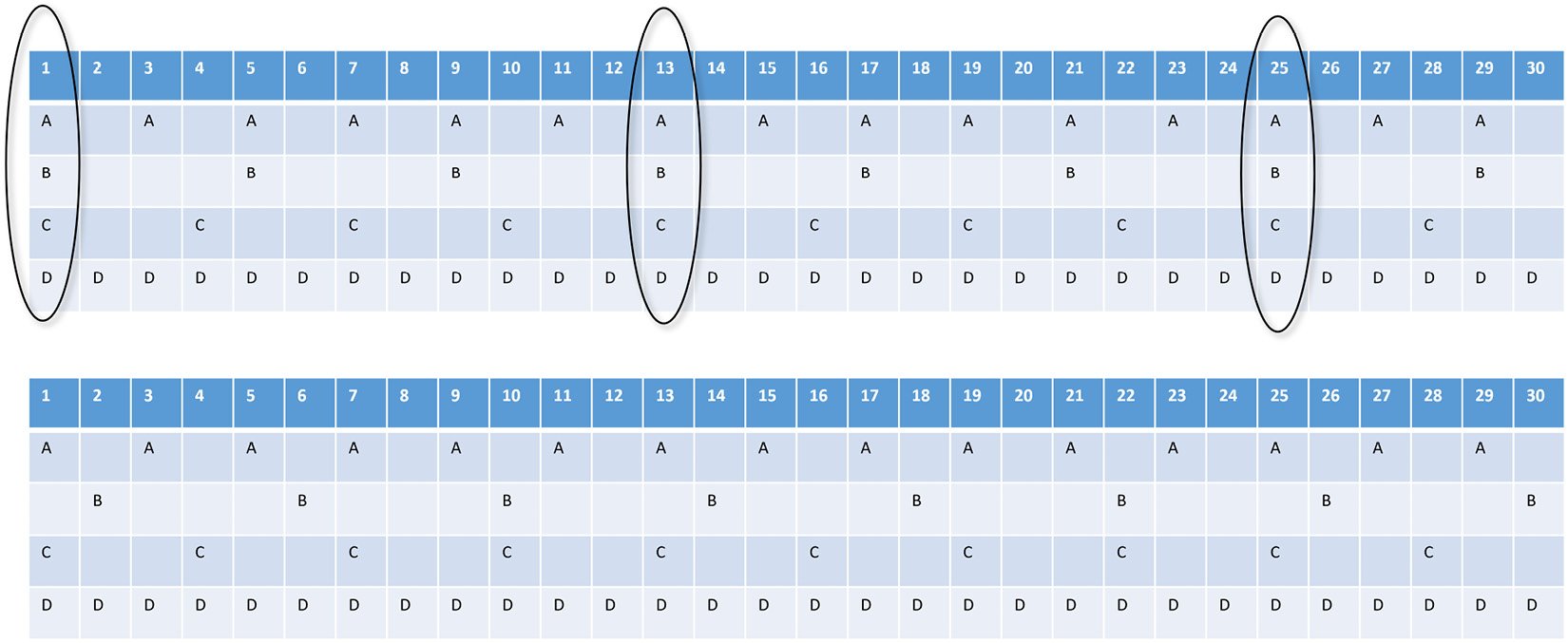
Figure 1.7 – Frame-based task schedule
Our first pass (the top of the figure) at the schedule has all four tasks landing on the same frame at frames 1, 13, and 25. We can improve the balance of the load on the control program if we delay the start of task B on the second frame as shown in the bottom half of the diagram.
This is akin to how measures in music work, where a measure is a certain amount of time, and different notes have different intervals – one whole note can only appear once per measure, a half note can appear twice, all the way down to 64th notes. Just like a composer makes sure that each measure has the right number of beats, we can make sure that our control loop has a balanced measure of processes to execute each frame.
Let’s start by writing a little program to control our timing loop and to let you play with these principles.
This is exciting – our first bit of coding together. This program just demonstrates the timing control loop we are going to use in the main robot control program and is here to let you play around with some parameters and see the results. This is the simplest version I think is possible of a soft time-controlled loop, so feel free to improve and embellish it. I’ve made you a flowchart to help you understand this a little better:
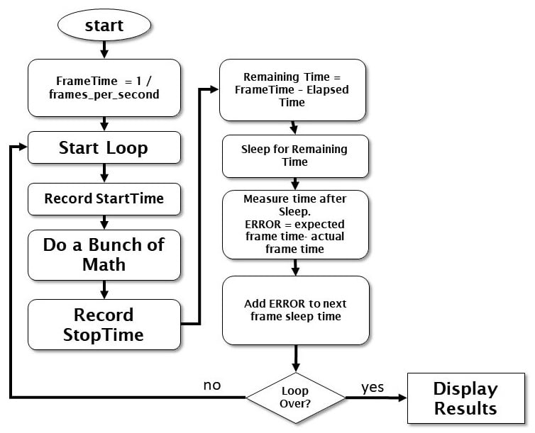
Figure 1.8 – Flowchart of soft real-time controller
Let’s look more closely at the terms used in the preceding diagram:
- FrameTime: The time we have allocated to execute one iteration of the loop
- StartTime: When the loop/frame begins
- Do a Bunch of Math: The program that you are managing
- StopTime: When the frame completes
- Remaining Time: The difference between the elapsed time and the desired frame time
- Elapsed Time: The time it takes to actually run through the loop once
- Frame Sleep Time: We use Remaining Time to tell the computer to sleep so that the frame takes exactly the amount of time we want.
Now we’ll begin with coding. This is pretty straightforward Python code – we won’t get fancy until later:
- We start by importing our libraries. It is not surprising that we start with the
timemodule. We also will use themeanfunction fromnumpy(Python numerical analysis) andmatplotlibto draw our graph at the end. We will also be doing some math calculations to simulate our processing and create a load on the frame rate:import time from numpy import mean import matplotlib.pyplot as plt import math #
- Now we have some parameters to control our test. This is where you can experiment with different timings. Our basic control is
FRAMERATE– how many updates per second do we want to try? Let’s start with30, as we did in the example we discussed earlier:# set our frame rate - how many cycles per second to run our loop? FRAMERATE = 30 # how long does each frame take in seconds? FRAME = 1.0/FRAMERATE # initialize myTimer # This is one of our timer variables where we will store the clock time from the operating system. myTimer = 0.0
- The duration of the test is set by the
countervariable. The time the test will take is theFRAMEtime times the number of cycles incounter. In our example, 2,000 frames divided by 30 fps is 66.6 seconds, or a bit over a minute to run the test:# how many cycles to test? counter*FRAME = runtime in seconds counter = 2000
We will be controlling our timing loop in two ways:
- We will first measure the amount of time it takes to perform the calculations for this frame. We have a stub of a program with some trigonometry functions we will call to put a load on the computer. Robot control functions, such as computing the angles needed in a robot arm, need lots of trig to work. This is available from
import mathin the header of the program.
- We will first measure the amount of time it takes to perform the calculations for this frame. We have a stub of a program with some trigonometry functions we will call to put a load on the computer. Robot control functions, such as computing the angles needed in a robot arm, need lots of trig to work. This is available from
Note
We will measure the time for our control function to run, which will take some part of our frame. We then compute how much of our frame remains, and tell the computer to sleep this process for the rest of the time. Using the sleep function releases the computer to go and take care of other business in the operating system, and is a better way to mark time rather than running a tight loop of some sort to waste the rest of our frame time.
- The second way we control our loop is by measuring the complete frame – compute time plus rest time – and looking to see whether we are over or under our frame time. We use
TIME_CORRECTIONfor this function to trim our sleep time to account for variability in the sleep function and any delays getting back from the operating system:# factor for our timing loop computations TIME_CORRECTION= 0.0
- We will collect some data to draw a jitter graph at the end of the program. We use the
dataStorestructure for this. Let’s put a header on the screen to tell you the program has begun, since it takes a while to finish:# place to store data dataStore = [] # Operator information ready to go # We create a heading to show that the program is starting its test print "START COUNTING: FRAME TIME", FRAME, "RUN TIME:",FRAME*counter
- In this step, we are going to set up some variables to measure our timing. As we mentioned, the objective is to have a bunch of compute frames, each the same length. Each frame has two parts: a compute part, where we are doing work, and a sleep period, when we are allowing the computer to do other things.
myTimeis the top of frame time, when the frame begins.newTimeis the end of the work period timer. We usemasterTimeto compute the total time the program is running:# initialize the precision clock myTime = newTime = time.time() # save the starting time for later masterTime=myTime # begin our timing loop for ii in range(counter):
- This section is our payload – the section of the code doing the work. This might be an arm angle calculation, a state estimate, or a command interpreter. We’ll stick in some trig functions and some math to get the CPU to do some work for us. Normally, this working section is the majority of our frame, so let’s repeat these math terms 1,000 times:
    # we start our frame - this represents doing some detailed
    math calculations
    # this is just to burn up some CPU cycles
    for jj in range(1000):
          x = 100
          y = 23 + ii
          z = math.cos(x)
          z1 = math.sin(y)
    #
    # read the clock after all compute is done
    # this is our working frame time
    #
- Now we read the clock to find the working time. We can now compute how long we need to sleep the process before the next frame. The important part is that working time + sleep time = frame time. I’ll call this
timeError:newTime = time.time() # how much time has elapsed so far in this frame # time = UNIX clock in seconds # so we have to subract our starting time to get the elapsed time myTimer = newTime-myTime # what is the time left to go in the frame? timeError = FRAME-myTimer
We carry forward some information from the previous frame here.
TIME_CORRECTIONis our adjustment for any timing errors in the previous frame time. We initialized it earlier to zero before we started our loop so we don’t get an undefined variable error here. We also do some range checking because we can get some large jitters in our timing caused by the operating system that can cause our sleep timer to crash if we try to sleep a negative amount of time:
Note
We use the Python max function as a quick way to clamp the value of sleep time to be zero or greater. It returns the greater of two arguments. The alternative is something like if a< 0 : a=0.
    # OK time to sleep
    # the TIME CORRECTION helps account for all of this clock
    reading
    # this also corrects for sleep timer errors
    # we are using a porpotional control to get the system to
    converge
    # if you leave the divisor out, then the system oscillates
    out of control
    sleepTime = timeError + (TIME_CORRECTION/2.0)
    # quick way to eliminate any negative numbers
    # which are possible due to jitter
    # and will cause the program to crash
    sleepTime=max(sleepTime,0.0)
- So, here is our actual sleep command. The
sleepcommand does not always provide a precise time interval, so we will be checking for errors:# put this process to sleep time.sleep(sleepTime)
- This is the time correction section. We figure out how long our frame time was in total (working and sleeping) and subtract it from what we want the frame time to be (
FrameTime). Then we set our time correction to that value. I’m also going to save the measured frame time into a data store so we can graph how we did later usingmatplotlib. This technique is one of Python’s more useful features:#print timeError,TIME_CORRECTION # set our timer up for the next frame time2=time.time() measuredFrameTime = time2-myTime ##print measuredFrameTime, TIME_CORRECTION=FRAME-(measuredFrameTime) dataStore.append(measuredFrameTime*1000) #TIME_CORRECTION=max(-FRAME,TIME_CORRECTION) #print TIME_CORRECTION myTime = time.time()
This completes the looping section of the program. This example does 2,000 cycles of 30 frames a second and finishes in 66.6 seconds. You can experiment with different cycle times and frame rates.
- Now that we have completed the program, we can make a little report and a graph. We print out the frame time and total runtime, compute the average frame time (total time/counter), and display the average error we encountered, which we can get by averaging the data in
dataStore:# Timing loop test is over - print the results # # get the total time for the program endTime = time.time() - masterTime # compute the average frame time by dividing total time by our number of frames avgTime = endTime / counter #print report print "FINISHED COUNTING" print "REQUESTED FRAME TIME:",FRAME,"AVG FRAME TIME:",avgTime print "REQUESTED TOTAL TIME:",FRAME*counter,"ACTUAL TOTAL TIME:", endTime print "AVERAGE ERROR",FRAME-avgTime, "TOTAL_ERROR:",(FRAME*counter) - endTime print "AVERAGE SLEEP TIME: ",mean(dataStore),"AVERAGE RUN TIME",(FRAME*1000)-mean(dataStore) # loop is over, plot result # this lets us see the "jitter" in the result plt.plot(dataStore) plt.show()
The results from our program are shown in the following code block. Note that the average error is just 0.00018 of a second, or 0.18 milliseconds out of a frame of 33 milliseconds:
START COUNTING: FRAME TIME 0.0333333333333 RUN TIME: 66.6666666667
FINISHED COUNTING
REQUESTED FRAME TIME: 0.0333333333333 AVG FRAME TIME: 0.0331549999714
REQUESTED TOTAL TIME: 66.6666666667 ACTUAL TOTAL TIME: 66.3099999428
AVERAGE ERROR 0.000178333361944 TOTAL_ERROR: 0.356666723887
AVERAGE SLEEP TIME: 33.1549999714 AVERAGE RUN TIME 0.178333361944
The following figure shows the timing graph of our program:
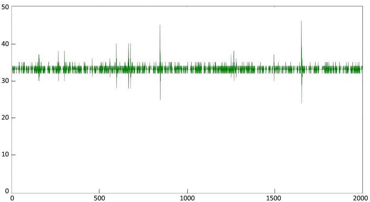
Figure 1.9 – Timing graph of our program
The spikes in the image are jitter caused by operating system interrupts. You can see the program controls the frame time in a fairly narrow range. If we did not provide control, the frame time would get greater and greater as the program executed. The graph shows that the frame time stays in a narrow range that keeps returning to the correct value.
Now that we have exercised our programming muscles, we can apply this knowledge to the main control loop for our robot with soft real-time control. This control loop has two primary functions:
- Respond to commands from the control station
- Interface to the robot’s motors and sensors in the Arduino Mega
We will discuss this in detail in Chapter 7.


