Importing Excel files
The read_excel method of the pandas library can be used to import data from an Excel file and load it into memory as a pandas DataFrame. In this recipe, we import an Excel file and handle some common issues when working with Excel files: extraneous header and footer information, selecting specific columns, removing rows with no data, and connecting to particular sheets.
Despite the tabular structure of Excel, which invites the organization of data into rows and columns, spreadsheets are not datasets and do not require people to store data in that way. Even when some data conforms with those expectations, there is often additional information in rows or columns before or after the data to be imported. Data types are not always as clear as they are to the person who created the spreadsheet. This will be all too familiar to anyone who has ever battled with importing leading zeros. Moreover, Excel does not insist that all data in a column be of the same type, or that column headings be appropriate for use with a programming language such as Python.
Fortunately, read_excel has a number of options for handling messiness in Excel data. These options make it relatively easy to skip rows, select particular columns, and pull data from a particular sheet or sheets.
Getting ready
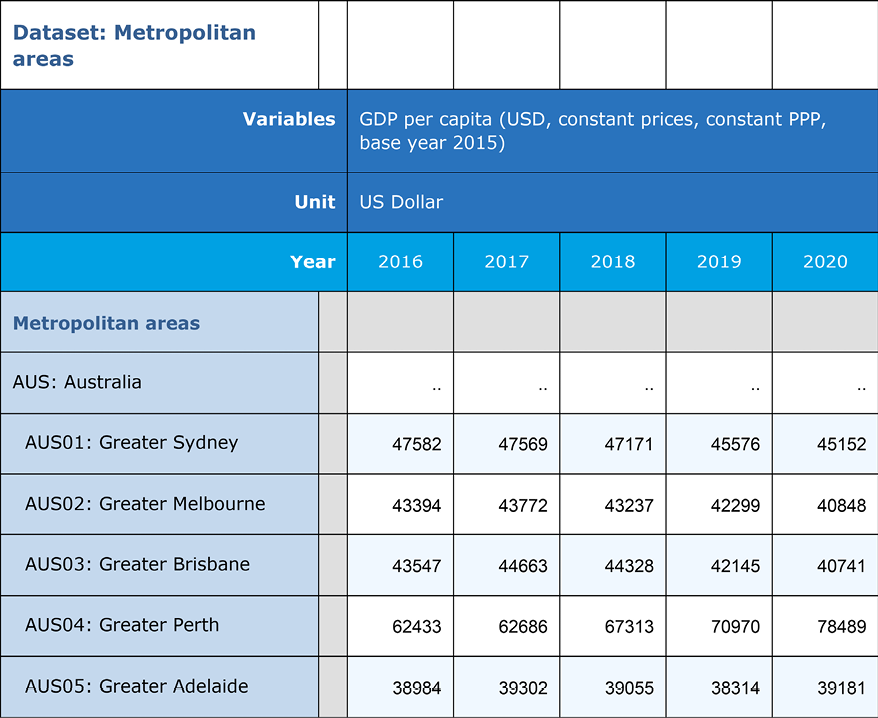
You can download the GDPpercapita22b.xlsx file, as well as the code for this recipe, from the GitHub repository for this book. The code assumes that the Excel file is in a data subfolder. Here is a view of the beginning of the file (some columns were hidden for display purposes):

Figure 1.2: View of the dataset
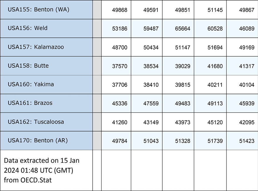
And here is a view of the end of the file:

Figure 1.3: View of the dataset
Data note
This dataset, from the Organisation for Economic Co-operation and Development, is available for public use at https://stats.oecd.org/.
How to do it…
We import an Excel file into pandas and do some initial data cleaning:
- Import the
pandaslibrary:import pandas as pd - Read the Excel per capita GDP data.
Select the sheet with the data we need, but skip the columns and rows that we do not want. Use the sheet_name parameter to specify the sheet. Set skiprows to 4 and skipfooter to 1 to skip the first four rows (the first row is hidden) and the last row. We provide values for usecols to get data from column A and columns C through W (column B is blank). Use head to view the first few rows and shape to get the number of rows and columns:
percapitaGDP = pd.read_excel("data/GDPpercapita22b.xlsx",
...    sheet_name="OECD.Stat export",
...    skiprows=4,
...    skipfooter=1,
...    usecols="A,C:W")
percapitaGDP.head()
                                  Year	2000	...	2019	2020
0	Metropolitan areas	       ...	NaN 	...	NaN	NaN
1	AUS: Australia	..	       ...	...  	...	...	...
2	AUS01: Greater Sydney	       ...	... 	... 	45576	45152
3	AUS02: Greater Melbourne     ...	... 	... 	42299	40848
4	AUS03: Greater Brisbane      ...	... 	... 	42145	40741
[5 rows x 22 columns]
percapitaGDP.shape
(731, 22)
Note
You may encounter a problem with read_excel if the Excel file does not use utf-8 encoding. One way to resolve this is to save the Excel file as a CSV file, reopen it, and then save it with utf-8 encoding.
- Use the
infomethod of the DataFrame to view data types and thenon-nullcount. Notice that all columns have theobjectdata type:percapitaGDP.info()<class 'pandas.core.frame.DataFrame'> RangeIndex: 731 entries, 0 to 730 Data columns (total 22 columns): # Column Non-Null Count Dtype --- ------ -------------- ----- 0 Year 731 non-null object 1 2000 730 non-null object 2 2001 730 non-null object 3 2002 730 non-null object 4 2003 730 non-null object 5 2004 730 non-null object 6 2005 730 non-null object 7 2006 730 non-null object 8 2007 730 non-null object 9 2008 730 non-null object 10 2009 730 non-null object 11 2010 730 non-null object 12 2011 730 non-null object 13 2012 730 non-null object 14 2013 730 non-null object 15 2014 730 non-null object 16 2015 730 non-null object 17 2016 730 non-null object 18 2017 730 non-null object 19 2018 730 non-null object 20 2019 730 non-null object 21 2020 730 non-null object dtypes: object(22) memory usage: 125.8+ KB - Rename the
Yearcolumn tometro, and remove the leading spaces.
Give an appropriate name to the metropolitan area column. There are extra spaces before the metro values in some cases. We can test for leading spaces with startswith(' ') and then use any to establish whether there are one or more occasions when the first character is blank. We can use endswith(' ') to examine trailing spaces. We use strip to remove both leading and trailing spaces. When we test for trailing spaces again, we see that there are none:
percapitaGDP.rename(columns={'Year':'metro'}, inplace=True)
percapitaGDP.metro.str.startswith(' ').any()
True
percapitaGDP.metro.str.endswith(' ').any()
False
percapitaGDP.metro = percapitaGDP.metro.str.strip()
percapitaGDP.metro.str.startswith(' ').any()
False
- Convert the data columns to numeric.
Iterate over all of the GDP year columns (2000–2020) and convert the data type from object to float. Coerce the conversion even when there is character data – the .. in this example. We want character values in those columns to become missing, which is what happens. Rename the year columns to better reflect the data in those columns:
for col in percapitaGDP.columns[1:]:
...   percapitaGDP[col] = pd.to_numeric(percapitaGDP[col],
...     errors='coerce')
...   percapitaGDP.rename(columns={col:'pcGDP'+col},
...     inplace=True)
...
percapitaGDP.head()
                      metro  pcGDP2000  pcGDP2001  ...  \
0        Metropolitan areas        NaN        NaN  ...
1            AUS: Australia        NaN        NaN  ...
2     AUS01: Greater Sydney        NaN      41091  ...
3  AUS02: Greater Melbourne        NaN      40488  ...
4   AUS03: Greater Brisbane        NaN      35276  ...
   pcGDP2018  pcGDP2019  pcGDP2020
0        NaN        NaN        NaN
1        NaN        NaN        NaN
2      47171      45576      45152
3      43237      42299      40848
4      44328      42145      40741
[5 rows x 22 columns]
percapitaGDP.dtypes
metro          object
pcGDP2000      float64
pcGDP2001      float64
abbreviated to save space
pcGDP2019      float64
pcGDP2020      float64
dtype: object
- Use the
describemethod to generate summary statistics for all numeric data in the DataFrame:percapitaGDP.describe()pcGDP2000 pcGDP2001 pcGDP2002 ... pcGDP2018 \ count 158 450 479 ... 692 mean 33961 38874 39621 ... 41667 std 15155 13194 13061 ... 17440 min 2686 7805 7065 ... 5530 25% 21523 30790 31064 ... 31322 50% 35836 38078 39246 ... 41428 75% 42804 46576 47874 ... 51130 max 95221 96941 98929 ... 147760 pcGDP2019 pcGDP2020 count 596 425 mean 42709 39792 std 18893 19230 min 5698 5508 25% 29760 24142 50% 43505 41047 75% 53647 51130 max 146094 131082 [8 rows x 21 columns] - Remove rows where all of the per capita GDP values are missing.
Use the subset parameter of dropna to inspect all columns, starting with the second column (it is zero-based) and going through to the last column. Use how to specify that we want to drop rows only if all of the columns specified in subset are missing. Use shape to show the number of rows and columns in the resulting DataFrame:
percapitaGDP.dropna(subset=percapitaGDP.columns[1:], how="all", inplace=True)
percapitaGDP.shape
(692, 22)
- Set the index for the DataFrame using the metropolitan area column.
Confirm that there are 692 valid values for metro and that there are 692 unique values, before setting the index:
percapitaGDP.metro.count()
692
percapitaGDP.metro.nunique()
692
percapitaGDP.set_index('metro', inplace=True)
percapitaGDP.head()
                          pcGDP2000  pcGDP2001  ...  \
metro                                           ...
AUS01: Greater Sydney           NaN      41091  ...
AUS02: Greater Melbourne        NaN      40488  ...
AUS03: Greater Brisbane         NaN      35276  ...
AUS04: Greater Perth            NaN      43355  ...
AUS05: Greater Adelaide         NaN      36081  ...
                          pcGDP2019  pcGDP2020
metro
AUS01: Greater Sydney         45576      45152
AUS02: Greater Melbourne      42299      40848
AUS03: Greater Brisbane       42145      40741
AUS04: Greater Perth          70970      78489
AUS05: Greater Adelaide       38314      39181
[5 rows x 21 columns]
percapitaGDP.loc['AUS02: Greater Melbourne']
pcGDP2000     NaN
pcGDP2001   40488
...
pcGDP2019   42299
pcGDP2020   40848
Name: AUS02: Greater Melbourne, dtype: float64
We have now imported the Excel data into a pandas DataFrame and cleaned up some of the messiness in the spreadsheet.
How it works…
We mostly manage to get the data we want in Step 2 by skipping rows and columns we do not want, but there are still a number of issues – read_excel interprets all of the GDP data as character data, many rows are loaded with no useful data, and the column names do not represent the data well. In addition, the metropolitan area column might be useful as an index, but there are leading and trailing blanks, and there may be missing or duplicated values.
read_excel interprets Year as the column name for the metropolitan area data because it looks for a header above the data for that Excel column and finds Year there. We rename that column metro in Step 4. We also use strip to fix the problem with leading and trailing blanks. We could have just used lstrip to remove leading blanks, or rstrip if there had been trailing blanks. It is a good idea to assume that there might be leading or trailing blanks in any character data, cleaning that data shortly after the initial import.
The spreadsheet authors used .. to represent missing data. Since this is actually valid character data, those columns get the object data type (that is how pandas treats columns with character or mixed data). We coerce a conversion to numeric type in Step 5. This also results in the original values of .. being replaced with NaN (not a number), how pandas represents missing values for numbers. This is what we want.
We can fix all of the per capita GDP columns with just a few lines because pandas makes it easy to iterate over the columns of a DataFrame. By specifying [1:], we iterate from the second column to the last column. We can then change those columns to numeric and rename them to something more appropriate.
There are several reasons why it is a good idea to clean up the column headings for the annual GDP columns – it helps us to remember what the data actually is; if we merge it with other data by metropolitan area, we will not have to worry about conflicting variable names; and we can use attribute access to work with pandas Series based on those columns, which I will discuss in more detail in the There’s more… section of this recipe.
describe in Step 6 shows us that fewer than 500 rows have valid data for per capita GDP for some years. When we drop all rows that have missing values for all per capita GDP columns in step 7, we end up with 692 rows in the DataFrame.
There’s more…
Once we have a pandas DataFrame, we have the ability to treat columns as more than just columns. We can use attribute access (such as percapitaGPA.metro) or bracket notation (percapitaGPA['metro']) to get the functionality of a pandas Series. Either method makes it possible to use Series string inspecting methods, such as str.startswith, and counting methods, such as nunique. Note that the original column names of 20## did not allow attribute access because they started with a number, so percapitaGDP.pcGDP2001.count() works, but percapitaGDP.2001.count() returns a syntax error because 2001 is not a valid Python identifier (since it starts with a number).
pandas is rich with features for string manipulation and for Series operations. We will try many of them out in subsequent recipes. This recipe showed those that I find most useful when importing Excel data.
See also
There are good reasons to consider reshaping this data. Instead of 21 columns of GDP per capita data for each metropolitan area, we should have 21 rows of data for each metropolitan area, with columns for year and GDP per capita. Recipes for reshaping data can be found in Chapter 11, Tidying and Reshaping Data.


