Search icon CANCEL
Subscription
0
Cart icon
Your Cart (0 item)
Close icon
You have no products in your basket yet
Save more on your purchases! discount-offer-chevron-icon
Savings automatically calculated. No voucher code required.
Arrow left icon
Explore Products
Best Sellers
New Releases
Books
Videos
Audiobooks
Learning Hub
Newsletter Hub
Free Learning
Arrow right icon
timer SALE ENDS IN
0 Days
:
00 Hours
:
00 Minutes
:
00 Seconds
Arrow up icon
GO TO TOP
Hands-On Markov Models with Python

You're reading from   Hands-On Markov Models with Python Implement probabilistic models for learning complex data sequences using the Python ecosystem

Arrow left icon
Product type Paperback
Published in Sep 2018
Publisher Packt
ISBN-13 9781788625449
Length 178 pages
Edition 1st Edition
Languages
Concepts
Arrow right icon
Authors (2):
Arrow left icon
Ankur Ankan Ankur Ankan
Author Profile Icon Ankur Ankan
Ankur Ankan
Abinash Panda Abinash Panda
Author Profile Icon Abinash Panda
Abinash Panda
Arrow right icon
View More author details
Toc

Markov chains or discrete-time Markov processes

A Markov chain is a type of Markov process in which the time is discrete. However, there is a lot of disagreement among researchers on what categories of Markov process should be called Markov chain. But, most commonly, it is used to refer to discrete-state-space Markov processes. Therefore, a Markov chain is a stochastic process over a discrete state space satisfying the Markov property. More formally, we can say that a discrete-time Markov chain is a sequence of random variables X1, X2, X3, ... that satisfy the Markov property, namely that the probability of moving from the current state to the next state depends only on the present state and not on any of the previous states. In terms of the probability distribution, we can say that, given that the system is at time instance n, the conditional distribution of the states at the next time instance, n + 1, is conditionally independent of the state of the system at time instances {1, 2, . . ., n-1}, given the state of the random variable at time instance n. This can be written as follows:

Markov chains are often represented using directed graphs. The nodes in the directed graphs represent the different possible states of the random variables, and the edges represent the probability of the system going from one state to the other in the next time instance. Let's take a simple example of predicting the weather to understand this representation better. We will consider that there are three possible states of the random variable Weather={Sunny, Rainy, Snowy}, and possible Markov chains for this can be represented as shown in Figure 1.1:
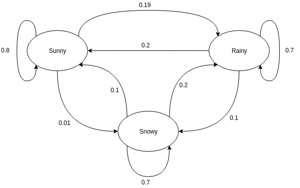
Figure 1.1: A simple Markov chain on the random variable, representing the random variable Weather={Sunny, Rainy, Snowy} and showing the probability of the random variable switching to other states in the next time instance

One of the main points to understand in Markov chains is that we are modeling the outcomes of a sequence of random variables over time. This is sometimes confusing for people since the model is represented using a single graph, which doesn't mention anything about time. So, the name state transitions is not a particularly good name for this, since the state is not changing for any random variable; rather, we are trying to determine the state of the next random variable given the observed state of our current random variable. Coming back to our example, we can see that the nodes of the graph represent the different possible states of the random variable Weather, and the edges between them show the probability of the next random variable taking the different possible states, given the state of the current random variable. The self-loops show the probability of the model staying in its current state. In the previous Markov chain, let's say we know that the observed state of the current random variable is Sunny, then the probability that the random variable at the next time instance will also take the value Sunny is 0.8. It could also take the value Rainy with a probability of 0.19, or Snowy with a probability of 0.01. One thing to note here is that the sum of all the probability values on all the outward edges from any state should equal 1, since it's an exhaustive event.

Now, let's try to code this simple Markov chain. We will start by defining a simple MarkovChain class, and we will keep on adding methods to this class as we go through this chapter:

import numpy as np

class MarkovChain(object):
def __init__(self, transition_prob):
"""
Initialize the MarkovChain instance.

Parameters
----------
transition_prob: dict
A dict object representing the transition probabilities in
Markov Chain. Should be of the form: {'state1': {'state1':
0.1, 'state2': 0.4}, 'state2': {...}}
"""
self.transition_prob = transition_prob
self.states = list(transition_prob.keys())

def next_state(self, current_state):
"""
Returns the state of the random variable at the next time
instance.

Parameters
----------
current_state: str
The current state of the system.
"""
return np.random.choice(
self.states, p=[self.transition_prob[current_state][next_state]
for next_state in self.states])

def generate_states(self, current_state, no=10):
"""
Generates the next states of the system.

Parameters
----------
current_state: str
The state of the current random variable.

no: int
The number of future states to generate.
"""
future_states = []
for i in range(no):
next_state = self.next_state(current_state)
future_states.append(next_state)
current_state = next_state
return future_states

Now, we can try out our example with this MarkovChain class:

>>> transition_prob = {'Sunny': {'Sunny': 0.8, 'Rainy': 0.19, 
'Snowy': 0.01},
'Rainy': {'Sunny': 0.2, 'Rainy': 0.7,
'Snowy': 0.1},
'Snowy': {'Sunny': 0.1, 'Rainy': 0.2,
'Snowy': 0.7}}

>>> weather_chain = MarkovChain(transition_prob=transition_prob)
>>> weather_chain.next_state(current_state='Sunny')
'Sunny'
>>> weather_chain.next_state(current_state='Snowy')
'Snowy'
>>> weather_chain.generate_states(current_state='Snowy', no=10)
['Snowy', 'Snowy', 'Snowy', 'Rainy', 'Snowy', 'Snowy', 'Rainy', 'Rainy', 'Snowy', 'Snowy']
In the previous code example, you might find your outputs to be different from what's shown here. This is because the Markov chain is probabilistic in nature and it picks on the next state based on a probability distribution, which can give different outputs on different runs.

So far in the discussion, we have considered that the probability space of the variables doesn't change over different instances of time. This is known as a time-homogeneous Markov chain, but it is also possible to have a time-inhomogeneous Markov chain, which also has a lot of applications but is outside the scope of this book.

Parameterization of Markov chains

In the code for the Markov chain in the previous section, we used a dictionary to parameterize the Markov chain that had the probability values of all the possible state transitions. Another way of representing state transitions is using a transition matrix. The transition matrix, as the name suggests, uses a tabular representation for the transition probabilities. The transition matrix for the example in Figure 1.1 is shown in the following table.

The following table shows the transition matrix for the Markov chain shown in Figure 1.1. The probability values represent the probability of the system going from the state in the row to the states mentioned in the columns:

States Sunny Rainy Snowy
Sunny 0.8 0.19 0.01
Rainy 0.2 0.7 0.1
Snowy 0.1+ 0.2 0.7

The transition matrix represents the same information as in the dictionary, but in a more compact way. For this reason, the transition matrix is the standard way of representing Markov chains. Let's modify our MarkovChain class so that it can accept a transition matrix:

import numpy as np

class MarkovChain(object):
def __init__(self, transition_matrix, states):
"""
Initialize the MarkovChain instance.

Parameters
----------
transition_matrix: 2-D array
A 2-D array representing the probabilities of change of
state in the Markov Chain.

states: 1-D array
An array representing the states of the Markov Chain. It
needs to be in the same order as transition_matrix.
"""
self.transition_matrix = np.atleast_2d(transition_matrix)
self.states = states
self.index_dict = {self.states[index]: index for index in
range(len(self.states))}
self.state_dict = {index: self.states[index] for index in
range(len(self.states))}

def next_state(self, current_state):
"""
Returns the state of the random variable at the next time
instance.

Parameters
----------
current_state: str
The current state of the system.
"""
return np.random.choice(
self.states,
p=self.transition_matrix[self.index_dict[current_state], :])

def generate_states(self, current_state, no=10):
"""
Generates the next states of the system.

Parameters
----------
current_state: str
The state of the current random variable.

no: int
The number of future states to generate.
"""
future_states = []
for i in range(no):
next_state = self.next_state(current_state)
future_states.append(next_state)
current_state = next_state
return future_states

Running this code should also give similar results to what we got in the previous section. Using a transition matrix might not seem like a good idea because it requires us to create extra variables to store the indices. But, in cases when we have hundreds of states, using a transition matrix is much more efficient than using the simple dictionary implementation. In the case of a transition matrix, we can simply use NumPy indexing to get the probability values in the next_state method, whereas we were looping over all the state names in the previous implementation:

>>> transition_matrix = [[0.8, 0.19, 0.01],
[0.2, 0.7, 0.1],
[0.1, 0.2, 0.7]]
>>> weather_chain = MarkovChain(transition_matrix=transition_matrix,
states=['Sunny', 'Rainy', 'Snowy'])
>>> weather_chain.next_state(current_state='Sunny')
'Sunny'
>>> weather_chain.next_state(current_state='Snowy')
'Sunny'
>>> weather_chain.generate_states(current_state='Snowy', no=10)
['Snowy', 'Rainy', 'Rainy', 'Rainy', 'Rainy', 'Rainy',
'Rainy', 'Rainy', 'Sunny', 'Sunny']

Properties of Markov chains

In this section, we will talk about the different properties of Markov chains, namely reducibility, periodicity, transience and recurrence, ergodicity, and steady-state analysis and limiting distributions. We will also try some simple examples of our MarkovChain class to show these properties.

Reducibility

A Markov chain is said to be irreducible if we can reach any state of the given Markov chain from any other state. In terms of states, state j is said to be accessible from another state i if a system that started at state i has a non-zero probability of getting to the state j. In more formal terms, state j is said to be accessible from state i if an integer nij ≥ 0 exists such that the following condition is met:

The nij here is basically the number of steps it takes to go from state i to j, and it can be different for different pairs of values for i and j. Also, for a given state i, if all the values for nij = 0, it means that all the states of the Markov chain are directly accessible from it. The accessibility relation is reflexive and transitive, but not necessary symmetric. We can take a simple example to understand this property:

Figure 1.2: An example of an irreducible Markov chain

In the previous example, it can be clearly seen that all of the states are accessible from all other states and hence are irreducible.

Note in the examples in Figure 1.2 and Figure 1.3 that we haven't represented edges if probability values are 0. This helps to keep the model less complicated and easier to read.

In the following example, we can see that state D is not accessible from A, B, or C. Also, state C is not accessible from either A or B. But all the states are accessible from state D, and states A and B are accessible from C:

Figure 1.3: An example of a reducible Markov chain

We can also add a couple of methods to our MarkovChain class to check which states in our chain are reachable and whether our chain is irreducible:

from itertools import combinations

def is_accessible(self, i_state, f_state):
"""
Check if state f_state is accessible from i_state.

Parameters
----------
i_state: str
The state from which the accessibility needs to be checked.

f_state: str
The state to which accessibility needs to be checked.
"""
reachable_states = [i_state]
for state in reachable_states:
if state == self.index_dict[f_state]:
return True
else:
reachable_states.append(np.nonzero(
self.transition_matrix[self.index_dict[i_state], :])[0])
return False

def is_irreducible(self):
"""
Check if the Markov Chain is irreducible.
"""
for (i, j) in combinations(self.states, self.states):
if not self.is_accessible(i, j):
return False
return True

Let's give our examples a try using the examples in Figure 1.2 and Figure 1.3:

>>> transition_irreducible = [[0.5, 0.5, 0, 0],
[0.25, 0, 0.5, 0.25],
[0.25, 0.5, 0, 0.25],
[0, 0, 0.5, 0.5]]
>>> transition_reducible = [[0.5, 0.5, 0, 0],
[0, 1, 0, 0],
[0.25, 0.5, 0, 0],
[0, 0, 0.25, 0.75]]
>>> markov_irreducible = MarkovChain(transition_matrix=transition_irreducible,
states=['A', 'B', 'C', 'D'])
>>> markov_reducible = MarkovChain(transition_matrix=transition_reducible,
states=['A', 'B', 'C', 'D'])
>>> markov_irreducible.is_accessible(i_state='A', f_state='D')
True
>>> markov_irreducible.is_accessible(i_state='B', f_state='D')
True
>>> markov_irreducible.is_irreducible()
True
>>> markov_reducible.is_accessible(i_state='A', f_state='D')
False
>>> markov_reducible.is_accessible(i_state='D', f_state='A')
True
>>> markov_reducible.is_accessible(i_state='C', f_state='D')
False
>>> markov_reducible.is_irreducible()
False

Periodicity

State i is said to have period k if any possible path to return to state i would be a multiple of k steps. Formally, it is defined like this:

Here, gcd means the greatest common divisor (GCD). Basically, k is the GCD of the length/number of steps of all possible paths from state i back to itself. If there are no possible paths from state i back to itself, then the period for it is not defined. We also need to note that k has nothing to do with the number of steps required to return to the starting state. For example, let's say that for any given state the number of steps required to return to it are (4, 6, 8, 12, 16). In this case k=2, but the minimum number of steps required to return is 4, and 2 doesn't even appear in the list of possible numbers of steps.

For any given state in the Markov chain, if k=1, the state is said to be aperiodic. A Markov chain is called aperiodic if all of its states are aperiodic. One major thing to note is that, in the case of an irreducible Markov chain, a single aperiodic state is enough to imply that all the states are aperiodic. Let's take a simple example and check the periodicity of different states:

Figure 1.4: Markov chain is also periodic

In the previous example, we can easily see that for state A the possible paths to return are A -> B -> C -> A or A -> B -> C -> D -> E -> C -> A. For these two paths, the path lengths are 3 and 6, respectively, and hence state A has a period of 3. Similarly, B, C, D, and E also each has a period of 3 in the Markov chain, and hence the Markov chain is also periodic:

Figure 1.5: Example of Markov Chain with aperiodic states.

In this example, we added a couple of extra edges, due to which the possible path lengths for A are now 3, 5, 7, ...; and for B are 2, 3, 4, 5, ... And, since the GCD of these path lengths is 1, states A and B are both now aperiodic. Similarly, we can compute the period of other nodes, each of which is also 1, and hence the Markov chain is also aperiodic.

Let's now add a couple of new methods to our MarkovChain class to compute the period of different states and check whether our model is aperiodic:

def get_period(self, state):
"""
Returns the period of the state in the Markov Chain.

Parameters
----------
state: str
The state for which the period needs to be computed.
"""
return gcd([len(i) for i in all_possible_paths])

def is_aperiodic(self):
"""
Checks if the Markov Chain is aperiodic.
"""
periods = [self.get_period(state) for state in self.states]
for period in periods:
if period != 1:
return False
return True

Let's now try out our methods on our examples. In this example, we will randomly assign probability values to different transitions:

>>> transition_periodic = [[0, 1, 0, 0, 0],
[0, 0, 1, 0, 0],
[0.5, 0, 0, 0.5, 0],
[0, 0, 0, 0, 1],
[0, 0, 1, 0, 0]]
>>> transition_aperiodic = [[0, 1, 0, 0, 0],
[0, 0, 1, 0, 0],
[0.5, 0.25, 0, 0.25, 0],
[0, 0, 0, 0, 1],
[0, 0, 0.5, 0.5, 0]]
>>> markov_periodic = MarkovChain(transition_matrix=transition_periodic,
states=['A', 'B', 'C', 'D', 'E'])
>>> markov_aperiodic = MarkovChain(transition_matrix=transition_aperiodic,
states=['A', 'B', 'C', 'D', 'E'])

>>> markov_periodic.get_period('A')
3
>>> markov_periodic.get_period('C')
3
>>> markov_aperiodic.is_periodic()
False

>>> markov_aperiodic.get_period('A')
1
>>> markov_aperiodic.get_period('B')
1
>>> markov_aperiodic.is_periodic()
True

Transience and recurrence

Given that we start at state i, it is called transient if there is a non-zero probability that we will never return to state i. To define this in more formal terms, let's consider a random variable Ti as the first return time to state i:

Let's now define another term, , as the probability of the system returns to state i after n steps:

Now we can define that any given state i is transient if the following condition is met:

In the preceding equation, we are basically checking whether the total sum of probabilities of returning to state i in step sizes less than is less than 1. If the total sum is less than 1, it would mean that the probability of Ti to be is greater than 0 which would mean that the state i is transient. The given state i is called recurrent if it is not transient:

Figure 1.6:

In the preceding example, we can see that states A and B are transient because A doesn't have any incoming edge. B does have an incoming edge, but it's incoming from another transient state and therefore it is also transient. Hence, once the system leaves state A or B, it won't be able to come back.

It is really simple to check whether a given state is transient or not. We can simply check whether there are any incoming edges from other states or not. If not, the state is transient. Let's write a simple method to check this for our MarkovChain class:

def is_transient(self, state):
"""
Checks if a state is transient or not.

Parameters
----------
state: str
The state for which the transient property needs to be checked.
"""
if all(self.transition_matrix[~self.index_dict[state], self.index_dict[state]] == 0):
return True
else:
return False

Now we can use this method in our example in Figure 1.6 to check which nodes are transient:

>>> transient_matrix = [[0, 0.5, 0.5, 0],
[0, 0, 0.25, 0.75],
[0, 0, 0, 1],
[0, 0, 0.5, 0.5]]
>>> transient_markov = MarkovChain(transition_matrix=transient_matrix,
states=['A', 'B', 'C', 'D']) >>> transient_markov.is_transient('A')
True
>>> transient_markov.is_transient('B')
True
>>> transient_markov.is_transient('C')
False

In the following subsections, we will talk about the statistical properties of the random variable Ti.

Mean recurrence time

The first-return time for the initial state i is also known as the hitting time. It was represented using the random variable Ti in the previous section. The mean recurrence time of state i is defined as its expected return time:

If the mean recurrence time, Mi, is finite, the state is called positive recurrent, otherwise it is called null recurrent.

Expected number of visits

As is evident from the name, the expected number of visits for any state i is the number of times the system is expected to be in that state. Also, a given state i is recurrent if and only if the expected number of visits to i is infinite:

Absorbing states

State i is said to be an absorbing state if it is impossible for a system to leave that state once it reaches it. For a state to be an absorbing state, the probability of staying in the same state should be 1, and all the other probabilities should be 0:

In a Markov chain, if all the states are absorbing, then we call it an absorbing Markov chain:

Figure 1.7: An example showing an absorbing state C, since the probability of transitioning from state C to C is 1

Again, we can add a very simple method to check for absorbing states in our MarkovChain class:

def is_absorbing(self, state):
"""
Checks if the given state is absorbing.

Parameters
----------
state: str
The state for which we need to check whether it's absorbing
or not.
"""
state_index = self.index_dict[state]
if self.transition_matrix[state_index, state_index]

We can again check whether our state in the example is absorbing by creating a Markov chain and using the is_absorbing method:

>>> absorbing_matrix = [[0, 1, 0],
[0.5, 0, 0.5],
[0, 0, 1]]
>>> absorbing_chain = MarkovChain(transition_matrix=absorbing_matrix,
states=['A', 'B', 'C'])
>>> absorbing_chain.is_absorbing('A')
False
>>> absorbing_chain.is_absorbing('C')
True

Ergodicity

State i is said to be ergodic if it is recurrent, has a period of 1, and has a finite mean recurrence time. If all the states of a Markov chain are ergodic, then it's an ergodic Markov chain. In general terms, a Markov chain is ergodic if there is a number N, such that any state in the system can be reached from any other state in any number of steps greater than or equal to the number N. Therefore, in the case of a fully connected transition matrix, where all transitions have a non-zero probability, this condition is fulfilled with N=1.

Steady-state analysis and limiting distributions

In a Markov chain, vector π is called the stationary distribution if ∀ j ∈ s satisfies the following conditions:

The stationary distribution is one of the most important properties of Markov chains, and we will talk about it in much more detail in later sections of this chapter.

You have been reading a chapter from
Hands-On Markov Models with Python
Published in: Sep 2018
Publisher: Packt
ISBN-13: 9781788625449
Register for a free Packt account to unlock a world of extra content!
A free Packt account unlocks extra newsletters, articles, discounted offers, and much more. Start advancing your knowledge today.
Unlock this book and the full library FREE for 7 days
Get unlimited access to 7000+ expert-authored eBooks and videos courses covering every tech area you can think of
Renews at $19.99/month. Cancel anytime
Banner background image