Fine Tuning Generated Insights
Now that you've generated a few insights, it's important to fine-tune your results to cater to the business. This can involve small changes like renaming columns or relatively big ones like turning a set of rows into columns. pandas provides ample tools that help you fine-tune your data so that you can extract insights from it that are more comprehensible and valuable to the business. Let's examine a few of them in the section that follows.
Selecting and Renaming Attributes
At times, you might notice variances in certain attributes of your dataset. You may want to isolate those attributes so that you can examine them in greater detail. The following functions come in handy for performing such tasks:
- loc[label]: This method selects rows and columns by a label or by a boolean condition.
- loc[row_labels, cols]: This method selects rows present in row_labels and their values in the cols columns.
- iloc[location]: This method selects rows by integer location. It can be used to pass a list of row indices, slices, and so on.
In the sales DataFrame you can use the loc method to select, based on a certain condition, the values of Revenue, Quantity, and Gross Profit columns:
sales.loc[sales['Retailer country']=='United States', \
['Revenue', 'Quantity', 'Gross profit']].head()
This code selects values from the Revenue, Quantity, and Gross profit columns only if the Retailer country is the United States. The output of the first five rows should be:

Figure 2.29: Sub-selecting observations and attributes in pandas
Let's also learn about iloc. Even though you won't be using it predominantly in your analysis, it is good to know how it works. For example, in the sales DataFrame, you can select the first two rows (0,1) and the first 3 columns (0,1,2) using the iloc method as follows.
sales.iloc[[0,1],[0,1,2]]
This should give you the following output:

Figure 2.30: Sub-selecting observations using iloc
At times, you may find that the attributes of your interest might not have meaningful names, or, in some cases, they might be incorrectly named as well. For example, Profit may be named as P&L, making it harder to interpret. To address such issues, you can use the rename function in pandas to rename columns as well as the indexes.
The rename function takes a dictionary as an input, which contains the current column name as a key and the desired renamed attribute name as value. It also takes the axis as a parameter, which denotes whether the index or the column should be renamed.
The syntax of the function is as follows.
df.rename({'old column name':'new column name'},axis=1)
The preceding code will change the 'old column name' to 'new column name'. Here, axis=1 is used to rename across columns. The following code renames the Revenue column to Earnings:
sales=sales.rename({'Revenue':'Earnings'}, axis = 1)
sales.head()
Since we're using the parameter axis=1, we are renaming across columns. The resulting DataFrame will now be:
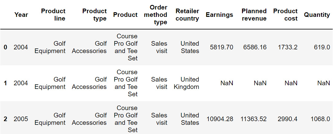
Figure 2.31: Output after using the rename function on sales
Note
The preceding image does not show all the rows of the output.
From the preceding output, you can observe that the Revenue column is now represented as Earnings. In the next section, we will understand how to transform values numerical values into categorical ones and vice versa.
Up until this chapter, we've been using the sales.csv dataset and deriving insights from it. Now, in the upcoming section and exercise, we will be working on another dataset (we will revisit sales.csv in Exercise 2.03, Visualizing Data with pandas).
In the next section, we will be looking at how to reshape data as well as its implementation.
Reshaping the Data
Sometimes, changing how certain attributes and observations are arranged can help understand the data better, focus on the relevant parts, and extract more information.
Let's consider the data present in CTA_comparison.csv. The dataset consists of Click to Action data of various variants of ads for a mobile phone along with the corresponding views and sales. Click to Action (CTA) is a marketing terminology that prompts the user for some kind of response.
Note
You can find the CTA_comparison.csv file here: https://packt.link/RHxDI.
Let's store the data in a DataFrame named cta as follows:
cta = pd.read_csv('CTA_comparison.csv')
cta
Note
Make sure you change the path (highlighted) to the CSV file based on its location on your system. If you're running the Jupyter Notebook from the same directory where the CSV file is stored, you can run the preceding code without any modification.
You should get the following DataFrame:
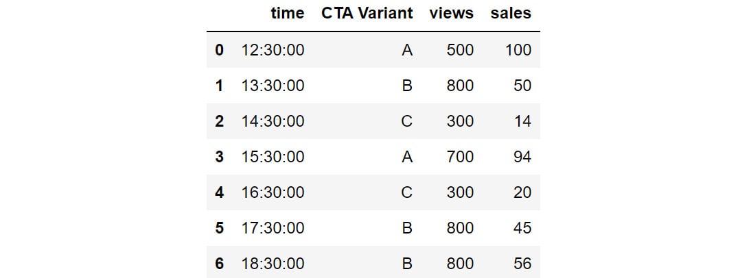
Figure 2.32: Snapshot of the data in CTA_comparison.csv
Notes
The outputs in Figure 2.32, Figure 2.33, and Figure 2.34 are truncated. These are for demonstration purposes only.
The DataFrame consists of CTA data for various variants of the ad along with the corresponding timestamps.
But, since we need to analyze the variants in detail, the CTA Variant column should be the index of the DataFrame and not time. For that, we'll need to reshape the data frame so that CTA Variant becomes the index. This can be done in pandas using the set_index function.
You can set the index of the cta DataFrame to CTA Variant using the following code:
cta.set_index('CTA Variant')
The DataFrame will now appear as follows:
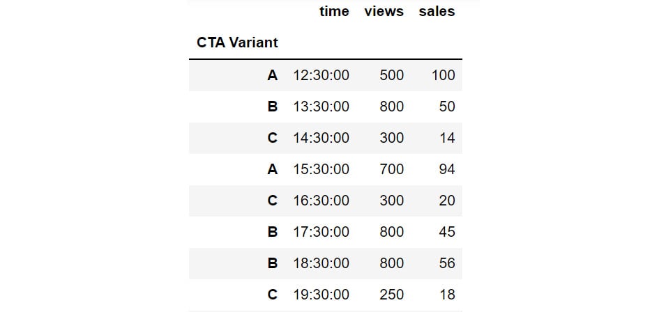
Figure 2.33: Changing the index with the help of set_index
You can also reshape data by creating multiple indexes. This can be done by passing multiple columns to the set_index function. For instance, you can set the CTA Variant and views as the indexes of the DataFrame as follows:
cta.set_index(['CTA Variant', 'views'])
The DataFrame will now appear as follows:
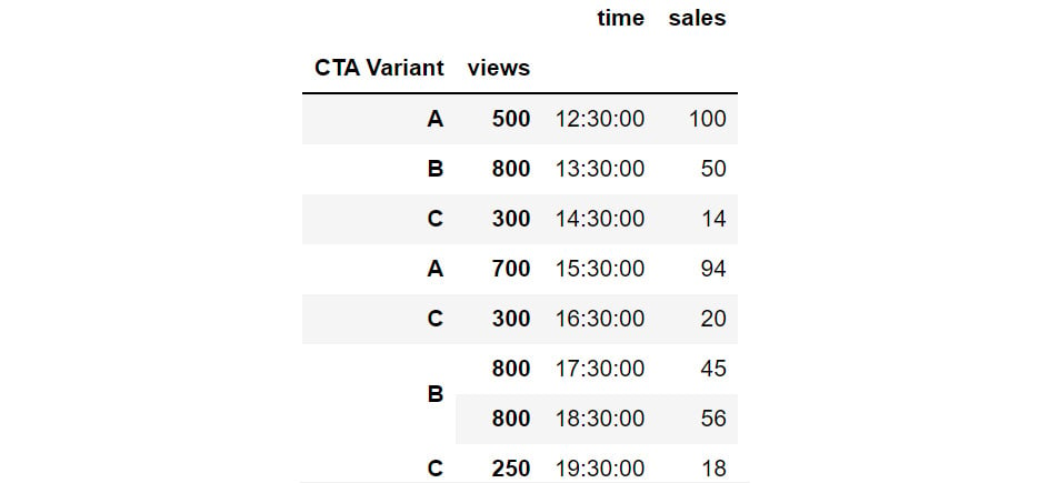
Figure 2.34: Hierarchical Data in pandas through set_index
In the preceding figure, you can see that CTA Variant and views are set as indexes. The same hierarchy can also be created, by passing multiple columns to the groupby function:
cta_views = cta.groupby(['CTA Variant', 'views']).count()
cta_views
This gives the following output:

Figure 2.35: Grouping by multiple columns to generate hierarchies
Using this hierarchy, you can see that CTA Variant B with 800 views is present thrice in the data.
Sometimes, switching the indices from rows to columns and vice versa can reveal greater insights into the data. This reshape transformation is achieved in pandas by using the unstack and stack functions:
- unstack(level): This function moves the row index with the name or integral location level to the innermost column index. By default, it moves the innermost row:
h1 = cta_views.unstack(level = 'CTA Variant')
h1
This gives the following output:

Figure 2.36: Example of unstacking DataFrames
You can see that the row index has changed to only views while the column has got the additional CTA Variant attribute as an index along with the existing time and sales columns.
- stack(level): This function moves the column index with the name or integral location level to the innermost row index. By default, it moves the innermost column:
h1.stack(0)
This gives the following output:

Figure 2.37: Example of stacking a DataFrame
Now the stack function has taken the other sales and time column values to the row index and only the CTA Variant feature has become the column index.
In the next exercise, you will implement stacking and unstacking with the help of a dataset.
Exercise 2.02: Calculating Conversion Ratios for Website Ads.
You are the owner of a website that randomly shows advertisements A or B to users each time a page is loaded. The performance of these advertisements is captured in a simple file called conversion_rates.csv. The file contains two columns: converted and group. If an advertisement succeeds in getting a user to click on it, the converted field gets the value 1, otherwise, it gets 0 by default; the group field denotes which ad was clicked – A or B.
As you can see, comparing the performance of these two ads is not that easy when the data is stored in this format. Use the skills you've learned so far, store this data in a data frame and modify it to show, in one table, information about:
- The number of views ads in each group got.
- The number of ads converted in each group.
- The conversion ratio for each group.
Note
You can find the conversion_rates.csv file here: https://packt.link/JyEic.
- Open a new Jupyter Notebook to implement this exercise. Save the file as Exercise2-02.ipnyb. Import the pandas library using the import command, as follows:
import pandas as pd
- Create a new pandas DataFrame named data and read the conversion_rates.csv file into it. Examine if your data is properly loaded by checking the first few values in the DataFrame by using the head() command:
data = pd.read_csv('conversion_rates.csv')
data.head()
Note
Make sure you change the path (highlighted) to the CSV file based on its location on your system. If you're running the Jupyter Notebook from the same directory where the CSV file is stored, you can run the preceding code without any modification.
You should get the following output:

Figure 2.38: The first few rows of conversion_rates.csv
- Group the data by the group column and count the number of conversions. Store the result in a DataFrame named converted_df:
converted_df = data.groupby('group').sum()
converted_df
You will get the following output:

Figure 2.39: Count of converted displays
From the preceding output, you can see that group A has 90 people who have converted. This means that advertisement A is quite successful compared to B.
- We would like to find out how many people have viewed the advertisement. For that use the groupby function to group the data and the count() function to count the number of times each advertisement was displayed. Store the result in a DataFrame viewed_df. Also, make sure you change the column name from converted to viewed:
viewed_df = data.groupby('group').count()\
.rename({'converted':'viewed'}, \
axis = 'columns')
viewed_df
You will get the following output:

Figure 2.40: Count of number of views
You can see that around 1030 people viewed advertisement A and 970 people viewed advertisement B.
- Combine the converted_df and viewed_df datasets in a new DataFrame, named stats using the following commands:
stats = converted_df.merge(viewed_df, on = 'group')
stats
This gives the following output:

Figure 2.41: Combined dataset
From the preceding figure, you can see that group A has 1030 people who viewed the advertisement, and 90 of them got converted.
- Create a new column called conversion_ratio that displays the ratio of converted ads to the number of views the ads received:
stats['conversion_ratio'] = stats['converted']\
/stats['viewed']
stats
This gives the following output:

Figure 2.42: Adding a column to stats
From the preceding figure, you can see that group A has a better conversion factor when compared with group B.
- Create a DataFrame df where group A's conversion ratio is accessed as df['A'] ['conversion_ratio']. Use the stack function for this operation:
df = stats.stack()
df
This gives the following output:

Figure 2.43: Understanding the different levels of your dataset
From the preceding figure, you can see the group-wise details which are easier to understand.
- Check the conversion ratio of group A using the following code:
df['A']['conversion_ratio']
You should get a value of 0.08738.
- To bring back the data to its original form we can reverse the rows with the columns in the stats DataFrame with the unstack() function twice:
stats.unstack().unstack()
This gives the following output:

Figure 2.44: Reversing rows with columns
This is exactly the information we needed in the goal of the exercise, stored in a neat, tabulated format. It is clear by now that ad A is performing much better than ad B given its better conversion ratio.
In this exercise, you have reshaped the data in a readable format. pandas also provides a simpler way to reshape the data that allows making comparisons while analyzing data very easy. Let's have a look at it in the next section.
Pivot Tables
A pivot table can be used to summarize, sort, or group data stored in a table. You've already seen an example of the pivot table functionality in excel; this one's similar to that. With a pivot table, you can transform rows to columns and columns to rows. The pivot function is used to create a pivot table. It creates a new table, whose row and column indices are the unique values of the respective parameters.
For example, consider the data DataFrame you saw in Step 2 of the preceding exercise:

Figure 2.45: The first few rows of the dataset being considered
You can use the pivot function to change the columns to rows as follows:
data=data.pivot(columns = 'group', values='converted')
data.head()
This gives the following output:

Figure 2.46: Data after being passed through the pivot command
In the preceding figure, note that the columns and indices have changed but the observations individually have not. You can see that the data that had either a 0 or 1 value remains as it is, but the groups that were not considered have their remaining values filled in as NaN.
There is also a function called pivot_table, which aggregates fields together using the function specified in the aggfunc parameter and creates outputs accordingly. It is an alternative to aggregations such as groupby functions. For instance, if we apply the pivot_table function to the same DataFrame to aggregate the data:
data.pivot_table(index='group', columns='converted', aggfunc=len)
This gives the following output:

Figure 2.47: Applying pivot_table to data
Note that the use of the len argument results in columns 0 and 1 that show how many times each of these values appeared in each group. Remember that, unlike pivot, it is essential to pass the aggfunc function when using the pivot_table function.
In the next section, you will be learning how to understand your data even better by visually representing it.


