Search icon CANCEL
Subscription
0
Cart icon
Your Cart (0 item)
Close icon
You have no products in your basket yet
Arrow left icon
Explore Products
Best Sellers
New Releases
Books
Videos
Audiobooks
Learning Hub
Free Learning
Arrow right icon
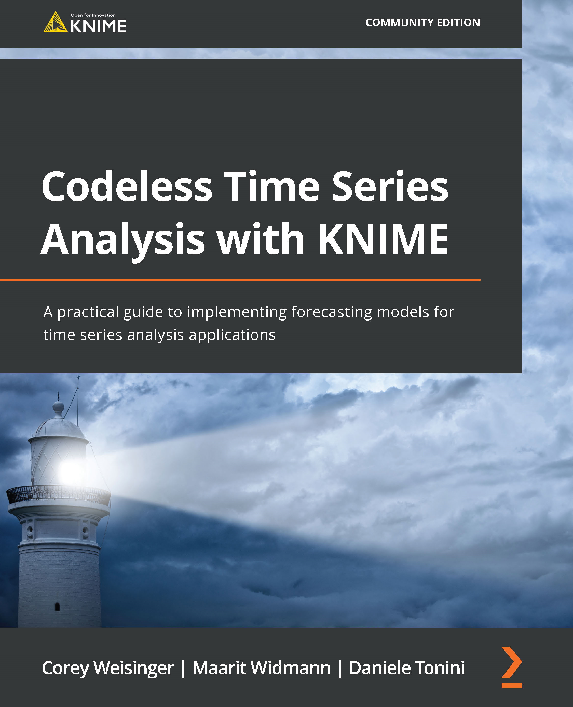
Codeless Time Series Analysis with KNIME

Codeless Time Series Analysis with KNIME: A practical guide to implementing forecasting models for time series analysis applications

Arrow left icon
Profile Icon Corey Weisinger Profile Icon KNIME AG Profile Icon Daniele Tonini Profile Icon Maarit Widmann
Arrow right icon
AU$14.99 AU$51.99
Full star icon Full star icon Full star icon Full star icon Half star icon 4.8 (10 Ratings)
eBook Aug 2022 392 pages 1st Edition
eBook
AU$14.99 AU$51.99
Paperback
AU$64.99
Subscription
Free Trial
Renews at AU$24.99p/m
eBook
AU$14.99 AU$51.99
Paperback
AU$64.99
Subscription
Free Trial
Renews at AU$24.99p/m

What do you get with eBook?

Product feature icon Instant access to your Digital eBook purchase
Product feature icon Download this book in EPUB and PDF formats
Product feature icon Access this title in our online reader with advanced features
Product feature icon DRM FREE - Read whenever, wherever and however you want
Product feature icon AI Assistant (beta) to help accelerate your learning
OR
Modal Close icon
Payment Processing...
tick Completed

Billing Address

Table of content icon View table of contents Preview book icon Preview Book

Codeless Time Series Analysis with KNIME

Chapter 1: Introducing Time Series Analysis

In this introductory chapter, we’ll examine the concept of time series, explore some examples and case studies, and then understand how Time Series Analysis (TSA) can be useful in different frameworks and applications. Finally, we’ll provide a brief overview of the forecasting models used over the years, highlighting their key features, which will be further explored in the following chapters.

In this chapter, we will cover the following topics:

  • Understanding TSA and its importance within data analytics
  • Time series properties and examples
  • TSA goals and applications
  • Overview of the main forecasting techniques used over the years

By the end of the chapter, you will have a good understanding of the key aspects of TSA, gaining the foundation to explore the subsequent chapters of the book with greater confidence.

Understanding TSA

When analyzing business data, it’s quite common to focus on what happened at a particular point in time: sales figures at the end of the month, customer characteristics at the end of the year, conversion results at the end of a marketing campaign, and more. Even in the development of the most sophisticated ML models, in most cases, we collect information that refers to different objects at a specific instant in time (or by taking a few snapshots of historical data). This approach, which is absolutely valid and correct for many applications, not only in business, uses cross-sectional data as the basis for analytics: data collected by observing many subjects (such as individuals, companies, shops, countries, equipment, and more) at one point or period of time.

Although the fact of not considering the temporal factor in the analysis is widespread and rooted in common practice, there are several situations where the analysis of the temporal evolution of a phenomenon provides more complete and interesting results. In fact, it’s only through the analysis of the temporal dynamics of the data that it is possible to identify the presence of some peculiar characteristics of the phenomenon we are analyzing, be it sales/consumption data, rather than a physical parameter or a macroeconomic index. These characteristics that act over time, such as trends, periodic fluctuations, level changes, anomalous observations, turning points, and more can have an effect in the short or long term, and often, it is important to be able to measure them precisely. Furthermore, it is only by analyzing data over time that it is possible to provide a reliable quantitative estimate of what might occur in the future (whether immediate or not). Since economic conditions are constantly changing over time, data analysts must be able to assess and predict the effects of these changes in order to suggest the most appropriate actions to take for the future.

For these reasons, TSA can be a very useful tool in the hands of business analysts and data scientists when it comes to both describing the patterns of a phenomenon along the time axis and providing a reliable forecast for it. Through the use of the right tools, TSA can significantly expand the understanding of any variable of interest (typically numerical) such as sales, financial KPIs, logistic metrics, sensors’ measurements, and more. More accurate and less biased forecasts that have been obtained through quantitative TSA can be one of the most effective drivers of performance in many fields and industries.

In the next sections of this chapter, we will provide definitions, examples, and some additional elements to gain a further understanding of how to recognize some key features of time series and how to approach their analyses in a structured way.

Exploring time series properties and examples

A general definition of a time series is the following:

A Time Series is a collection of observations made sequentially through time, whose dynamics are often characterized by short/long period fluctuations and/or long period direction.

This definition highlights two fundamental aspects of a time series: the fact that observations are a function of time and that, as a consequence of this fact, some typical temporal features are often observed. The fluctuations and the long period direction of the series are just some of these features, as there might be other relevant aspects to take into consideration such as autocorrelation, stationarity, and the order of integration. We will explore these aspects in more detail in future chapters. In this section, we will focus on the distinction between discrete time series and continuous time series, on the concept of independence between observations, and finally, we will show some examples of real-world time series.

Continuous and discrete time series

A Time Series is defined as continuous when observations are collected continuously over time, that is, there can be an infinite number of observations in a given time range. Typically, continuous time series data is sampled at irregular time intervals. Consider the measurement of a patient’s blood pressure in a hospital done at varying time points during the day, not equally spaced. This happens because, in some settings, regular monitoring at fixed intervals is not possible. For instance, in Figure 1.1, there are four medical continuous time series, relative to the health parameters of four patients:

  • Mean blood pressure
  • Heart rate
  • Temperature
  • Glucose data

As evident from the graphs, there are some temporal ranges where the measures are not present, for example, the temperature and glucose between approximately 20 hours and 30 hours of the monitoring period. There are other time points where data is collected more frequently than in other periods. These time series features are due to the fact that the data has been collected manually by the physician or by the nurse, not at fixed moments of the day. Therefore, this type of time series is inherently irregularly sampled:

Figure 1.1 – Four continuous, irregularly sampled, medical time series

Figure 1.1 – Four continuous, irregularly sampled, medical time series

A time series is defined as discrete when observations are collected regularly at specific times, typically equally spaced (that is, hourly, daily, weekly, and yearly data points).

A time series of this type can be natively discrete, such as the annual budget data of a company, or it can be created through the aggregation or accumulation of a numerical variable in equal time intervals. For example, the monthly sales of a supermarket or the number of daily passengers in a train station. A continuous time series can be discretized by binning/grouping the original data and, eventually, obtaining a discrete time series.

Classical TSA focuses on discrete time series because they are more common in real-world applications and easier to analyze. Therefore, in this book, we mainly deal with discrete time series, where observations are collected at equal intervals. When we consider irregularly sampled time series, first, we will try to transform them into regularly sampled data points.

Independence and serial correlation

One of the most distinctive characteristics of a time series is the mutual dependence between the observations, generally called serial correlation or autocorrelation.

In many statistical models, observations are assumed to be generated by a random sampling process and to be independent of each other (consider the linear regression model). Typically, this assumption turns out to be inconsistent with time series data, where simply collecting the data sequentially, along the time axis, generally produces observations that are not independent of each other.

Think of the daily sales of an e-commerce company. It’s reasonable to imagine that today’s sales are somehow related to the previous day’s sales: successive observations are dependent. However, in this context, which clearly can create some problems in using classical statistical tools, it is however possible to exploit the temporal dependence of observations to improve the forecasting process. If today’s sales are related to yesterday’s, and we can consistently estimate this relationship, then we can improve the forecast of tomorrow’s sales based on today’s result.

Time series examples

Interesting examples of time series can be collected in a multitude of information domains: business/economics, industrial production, social sciences, physics, and more. The time series obtained from these fields might be profoundly different in terms of statistical properties and the granularity of the available data, yet the methodologies of descriptive analysis and forecasting are essentially the same.

Here, we will explore a line chart (also called a time plot) of some representative discrete time series, with the aim of showing how it is possible to observe very different dynamics, depending on the type of data and the field of reference. Figure 1.2 shows the pattern of two annual time series, that is, the Number of PhDs awarded in the US, split between the subjects of engineering and education:

Figure 1.2 – Time series example 1: number of PhDs awarded in the US, showing the annual data for Engineering versus Education

Figure 1.2 – Time series example 1: number of PhDs awarded in the US, showing the annual data for Engineering versus Education

In the preceding graph, we can see that both time series do not show periodic fluctuations, and this is typical of annual data. The engineering doctorate series appears to be increasing over time, especially in the last 5 years presented, while the education doctorate series shows a flatter trend, with a level shift between 2010 and 2011.

Figure 1.3 – Time series example 2: monthly carbon dioxide concentration (globally averaged from marine surface sites)

Figure 1.3 – Time series example 2: monthly carbon dioxide concentration (globally averaged from marine surface sites)

Focusing on a different series, the Monthly carbon dioxide concentration in Figure 1.3 shows a completely different pattern than the previous series. In fact, the dynamics of this monthly time series are dominated by periodic fluctuations, which are repeated consistently every year. In addition, we observe the constant growth of the level of the carbon concentration, year after year. In summary, this series shows an increasing oscillatory pattern that appears to be quite stable and, therefore, easily predictable.

Figure 1.4 – Time series example 3: LinkedIn’s daily stock market closing price

Figure 1.4 – Time series example 3: LinkedIn’s daily stock market closing price

In contrast, the evolution of the time series shown in Figure 1.4 seems to be much more unpredictable. In this case, we have daily data points of LinkedIn’s stock market closing price. The pattern during the 5 years of observation seems to be very irregular, without periodic fluctuations, with sudden changes of direction superimposed on an increasing trend in the long run.

Figure 1.5 – Time series example 4: number of photos uploaded onto Instagram every minute (regional sub-sample)

Figure 1.5 – Time series example 4: number of photos uploaded onto Instagram every minute (regional sub-sample)

Considering another example in the social media theme, we can look at Figure 1.5, in which the plot shows the Number of photos uploaded onto Instagram every minute (regional sub-sample). In this case, the granularity of the data is very high (one observation every minute) and the dynamics of the time series show both elements of regularity, such as constant fluctuations and peaks that are observed in the early afternoon of each day. At the same time, there are also discontinuities such as the presence of some anomalous observations.

Figure 1.6 – Time series example 5: acceleration detected by smartphone sensors during a workout session (10 seconds)

Figure 1.6 – Time series example 5: acceleration detected by smartphone sensors during a workout session (10 seconds)

Finally, the analysis of the three time series shown in Figure 1.6, highlights how, for the same phenomenon (a workout session), both regular and irregular dynamics can be observed, depending on the point of observation. In this case, the three accelerometers mounted to the wearable device show fairly constant peaks along one spatial dimension and greater irregularity on the others.

In conclusion, from the examples that we have shown in this section, we notice that time series might have characteristics that are very different from one another. Determining aspects such as the origin of the data and the reference industry, the granularity of the data, and the length of the observation period can drastically influence the dynamics of the time series, revealing really heterogeneous patterns.

TSA goals and applications

When it comes to analyzing time series, depending on the industry and the type of project, different goals can be pursued, from the simplest to the most complex. Likewise, multiple analytical applications can be developed where TSA plays a crucial role. In this section, we will look at the main goals of time series analysis, followed by some examples of real-world applications.

Goals of TSA

In common practice, TSA is directly associated with forecasting, almost as if it were a synonym for this task. Although the objective of predicting the data for a future horizon is probably the most common (and challenging) goal, we should not assume TSA is only that. Often, the purpose of the analysis is to obtain a correct representation of data over time: think of the construction of a tool for data visualization and business intelligence or analyzing the data of a manufacturing process to detect possible anomalies.

Therefore, there are different objectives in the analysis of time series that can be listed in the following four points:

  • Exploratory analysis and visualization: This consists of the use of descriptive analytics tools dedicated to the summary of data points with respect to time. Through these analyses, it’s possible to identify the presence of specific temporal dynamics (for example, trends, seasonality, or cycles), detect outliers/gaps in the data, or search for a specific pattern. In business intelligence, it is critical to correctly represent time series within enterprise dashboards in order to provide immediate insights to business users for the decision-making process.
  • Causal effect discovery and simulation: In many sectors, often, it is useful to verify how one or more exogenous variables impact a target variable. For example, how advertising investments on different channels (whether digital or not) impact the sales of a company or how some environmental conditions impact the quality of the industrial production of a particular product. These types of problems are very common and, in data analytics, are frequently addressed through the estimation of multiple regression models (adapted to work well with time series data). Once possible causal relationships are identified, it is possible to simulate the outcome of the objective variable as a function of the values assumed by the exogenous variables.
  • Anomaly detection and process control (Figure 1.7): We can use TSA to prevent negative events (such as failures, damage, or performance drops):
Figure 1.7 – Anomaly detection using time series

Figure 1.7 – Anomaly detection using time series

The main idea is to promptly detect an anomaly during the operation of a device or the behavior of a subject, even if the specific anomaly has never been observed before. For many companies, reducing anomalies and improving quality is a key factor for growth and success; for example, reducing fraud in the banking sector or preventing cyber attacks in IT security systems. In manufacturing, process engineers use control charts to monitor the stability of a production process and also a measurement system. Typically, a control chart is obtained by plotting the data points of a time series related to a specific parameter of the manufacturing process (for example, wire pull strength, the concentration of a chemical, oxide thickness, and more) and adding some control limits, which is useful to identify possible process drifts or anomalies.

  • Forecasting: This definitely constitutes the main objective of time series analysis and consists of predicting the future values of a time series observed in the past. The forecasting horizon can be short-term or long-term. There are many methods used to obtain the predicted values; we will discuss these aspects in more detail in the Exploring Time series forecasting techniques section.

Domains of applications and use cases

The fields of application of TSA are numerous. Demand Forecasting and Planning is one of the most common applications, as it’s an important process for many companies (especially retailers) to anticipate demand for products throughout the entire supply chain, especially under uncertain conditions. However, from industry to industry, there are many more interesting uses of TSA. Right now, it would be almost impossible to list all applications where the use of TSA plays an important role in creating business solutions and assets; therefore, we will limit ourselves to a few examples that might give you an idea of the heterogeneity of use cases in the field of TSA.

For instance, consider the following list of examples:

  • Workforce planning: For a company operating in the logistics and transportation industry, it is crucial to predict the workload so that the right number of staff/couriers are available to handle it properly. In a workforce planning context, correctly forecasting the volume of parcels to be handled can help to effectively allocate effort and resources, which means eventually improving the bottom line for companies with, typically, low-profit margins.
  • Forecasting of sales during promotions: E-commerce, supermarkets, and retailers increasingly use promotions, discount periods, and special sales to increase sales volume; however, stock-out problems are often generated, resulting in customer dissatisfaction and extra operative costs. Therefore, it is essential to use forecasting models that integrate the effects of promotions into sales forecasting in order to optimize warehouses and avoid losses, both economic and reputational.
  • Insurance claim reserving: For insurance companies, estimating the claims reserve plays an important role in maintaining capital, determining premiums, and being in line with requirements imposed by the policyholder. Therefore, it is necessary to estimate the future number and amount of claims as correctly as possible. In recent years, actuarial practitioners have used several time series-based approaches to obtain reliable forecasts of claims and estimate the degree of uncertainty of the predictions.
  • Predictive maintenance: In the context of the Internet of Things, the availability of real-time information generated by sensors mounted on devices and manufacturing equipment enables the development of analytics solutions that can prevent negative events (such as failures, damage, or drops in performance) in order to improve the quality of products or reduce operating costs. Anomaly detection based on TSA is one of the most widely used methods for creating effective predictive maintenance solutions. In Chapter 11, Anomaly Detection – Predicting Failure with No Failure Examples, we will provide a detailed use case in this area.
  • Energy load forecasting: In deregulated energy markets, forecasting the consumption and price of electricity is crucial for defining effective bidding strategies to maximize a company’s profits. In this context, TSA is a widely used approach for day-ahead forecasting.

The applications just listed provide insight into how the application of TSA and forecasting techniques form the core of many processes and solutions developed in different industries.

Exploring time series forecasting techniques

Within the data science domain, doing time series forecasting first means extending a KPI (or any measure of interest) into the future in the most accurate and least biased way possible. And while this remains the primary goal of forecasting, often, the activity does not boil down to just that as it’s sometimes necessary to include an assessment of the uncertainty of forecasted values and comparisons with previous forecasting benchmarks. The approaches to time series forecasting are essentially two, listed as follows:

  • Qualitative forecasting methods are adopted when historical data is not available (for example, when estimating the revenues of a new company that clearly doesn’t have any data available). They are highly subjective methods. Among the most important qualitative forecasting techniques, it is possible to mention the Delphi method.
  • Quantitative forecasting techniques are based on historical quantitative data; the analyst/data scientist, starting from this data, tries to understand the underlying structure of the phenomenon of interest and then uses the same data for forecasting purposes. Therefore, the analyst’s task is to identify, isolate, and measure these temporal dynamics behind a time series of past data in order to make optimal predictions and eventually support decisions, planning, and business control. The quantitative approach to forecasting is certainly the most widely used, as it generates results that are typically more robust and more easily deployed into business processes. Therefore, from now on (including in the next chapters), we will focus exclusively on it.

In the following section, we will explore the details of quantitative forecasting, focusing on the basic requirements for carrying it out properly and the main quantitative techniques used in recent years.

Quantitative forecasting properties and techniques

First and foremost, the development of a quantitative forecasting model depends on the available data, both in terms of the amount of data and the quality of historical information. In general, we can say that there are two basic requirements for effectively creating a reliable quantitative forecasting model:

  • Obtain an adequate number of observations, which means a sufficient depth of historical data, in order to correctly understand the phenomenon under analysis, estimate the models, and then apply the predictions. Probably one of the most common questions asked by those who are facing the development of a forecasting model for the first time is how long does the Time Series need to be to obtain a reliable model, which, in simple terms, means how much past do I need? The answer is not simple. It would be incorrect to say at least 50 observations are needed or that the depth should be at least 5 years. In fact, the amount of data points to consider depends on the following:
    • The complexity of the model to be developed and the number of parameters to be estimated.
    • The amount of randomness in the data.
    • The granularity of the data (such as monthly, daily, and hourly) and its characteristics. (Is it intermittent? Are there strong periods of discontinuity to consider?)
    • The presence of one or more seasonal components that need to be estimated in relation to the granularity of the data (for example, to include a weekly seasonality pattern of hourly data in the model, at least several hundred observations must be available).
  • Collect information about the «time dimension» of the time series in order to determine the starting/ending points of the data and a possible length for the seasonal components (if present).

Given a set of sufficient historical data, the basis for a quantitative forecasting model is the assumption that there are factors that influenced the dynamics of the series in the past and these factors continue to bring similar effects in the future, too.

There are several criteria used to classify quantitative forecasting techniques. It is possible to consider the historical evolution of the methods (from the most classical to the most modern), how the methods use the information within the model, or even the domain of method development (purely statistical versus ML). Here, we present one possible classification of the techniques used for quantitative forecasting, which takes into account multiple relevant elements that characterize the different methods. We can consider these three main groups of methods as follows:

  1. Classical univariate forecasting methods: In these statistical techniques, the formation of forecasts is only based on the same time series to be forecast through the identification of structural components, such as trends and seasonality, and the study of the serial correlation. Some popular methods in this group are listed as follows:
    • Classical decomposition: This considers the observed series as the overlap of three elementary components (trend-cycle, seasonality, and residual), connected with different patterns that are typically present in many economics time series; classical decomposition (such as other types of decomposition) is a common way to explore and interpret the characteristics of a time series, but it can certainly be used to produce forecasts. In Chapter 5, Time Series Components and Statistical Properties, we will delve deeper into this method.
    • Exponential smoothing: Forecasts produced by exponential smoothing methods are based on weighted averages of past observations, with weights decaying exponentially as the observations get older; this decreasing weights method could also take into account the overlap of some components, such as trends and seasonality.
    • AutoRegressive Integrated Moving Average (ARIMA): Essentially, this is a regression-like approach that aims to model, as effectively as possible, the serial correlation among the observations in a time series. To do this effectively, several parameters in the model can handle trends and seasonality, although less directly than decomposition or exponential smoothing.
  2. Explanatory models: These techniques work in a multivariate fashion, so the forecasts are based on both past observations of the reference time series and external predictors, which helps to achieve better accuracy but also to obtain a more extensive interpretation of the model. The most popular example in this group is the ARIMAX model (or regression with ARIMA errors).
  3. ML methods: These techniques can be either univariate or multivariate. However, their most distinctive feature is that they originated outside the statistical domain and were not specifically designed to analyze time series data; typically, they are artificial neural networks (such as multilayer perceptron, long-short memory networks, and dilated convolutional neural networks) or tree-based algorithms (such as random forest or gradient boosted trees) originally made for cross-sectional data that can be adapted for time series forecasting.

A very common question asked by students and practitioners who are new to TSA is whether there is one forecasting method that is better than the others. The answer (for now) is no. All of the models have their own pros and cons. In general, exponential smoothing, ARIMA, and all the classical methodologies have been around the longest. They are quite easy to implement and typically very reliable, but they require the verification of some assumptions, and sometimes, they are not as flexible as you would like them to be. In contrast, ML algorithms are really flexible (they don’t have assumptions to check), but commonly, you need a large amount of data to train them properly. Moreover, they can be more complicated (a lot of hyperparameters to tune), and to be effective, you need to create some extra-temporal features to catch the time-related patterns within your data.

But what does the best forecasting model mean? Consider that it’s never just a matter of the pure performance of the model, as you need to consider other important items in the model selection procedure. For instance, consider the following list of items:

  • Forecast horizon in relation to TSA objectives: Are you going to predict the short term or the long term? For the same time series, you could have a model that is the best one for short-term forecasts, but you need to use another one for long-term forecasts.
  • The type/amount of available data: In general, for small datasets, a classical forecasting method could be better than an ML approach.
  • The required readability of the results: A classical model is more interpretable than an ML model.
  • The number of series to forecast: Using classical methods with thousands of time series can be inefficient, so in this case, an ML approach could be better.
  • Deployment-related issues: Also, consider the frequency of the delivery of the forecasts, the software environment, and the usage of the forecasts.

In summary, when facing the modeling part of your time series forecasting application, don’t just go with one algorithm. Try different approaches, considering your goals and the type/amount of data that you have.

Summary

In this chapter, we introduced TSA, starting by defining what a time series is and then providing some examples of series taken from various contexts and industries. Next, we focused on the goals that are typically related to TSA and also provided some examples of applications in real-world scenarios. Finally, we covered a brief review of the main forecasting methods, providing a taxonomy of methodologies and generally describing the characteristics of the main models, from the most classic to the most modern.

In this chapter, the basic concepts provided are of great importance for approaching the subsequent chapters of the book in a structured way, having the concepts of time series and forecasting clear in your head.

In the next chapter, we’ll cover the basic concepts of KNIME Analytics Platform and its time series integration, introducing the software and showing a first workflow example.

Questions

The answers to the following questions can be found in the Assessment section at the end of the book:

  1. What is a discrete Time Series?
    1. A collection of observations made continuously over time.
    2. A series where there can be an infinite number of observations in a given time range.
    3. A collection of observations that are sampled regularly at specific times, typically equally spaced.
    4. A series where observations follow a Bernoulli distribution.
  2. Which of the following is not a typical goal pursued in Time Series Analysis?
    1. Causal effect discovery and simulation.
    2. Function approximation.
    3. Anomaly detection and process control.
    4. Forecasting.
  3. Which is a basic requirement to develop a reliable quantitative forecasting model?
    1. Obtain an adequate number of historical observations.
    2. Collect time-independent observations.
    3. Collect a time series that shows a trend.
    4. Obtain a time series without gaps and outliers.
  4. Which of the following is not a group of methods typically used in quantitative Time Series Forecasting?
    1. Classical univariate methods.
    2. Machine learning techniques.
    3. Explanatory models.
    4. Direct clustering algorithms.
Left arrow icon Right arrow icon
Download code icon Download Code

Key benefits

  • Gain a solid understanding of time series analysis and its applications using KNIME
  • Learn how to apply popular statistical and machine learning time series analysis techniques
  • Integrate other tools such as Spark, H2O, and Keras with KNIME within the same application

Description

This book will take you on a practical journey, teaching you how to implement solutions for many use cases involving time series analysis techniques. This learning journey is organized in a crescendo of difficulty, starting from the easiest yet effective techniques applied to weather forecasting, then introducing ARIMA and its variations, moving on to machine learning for audio signal classification, training deep learning architectures to predict glucose levels and electrical energy demand, and ending with an approach to anomaly detection in IoT. There’s no time series analysis book without a solution for stock price predictions and you’ll find this use case at the end of the book, together with a few more demand prediction use cases that rely on the integration of KNIME Analytics Platform and other external tools. By the end of this time series book, you’ll have learned about popular time series analysis techniques and algorithms, KNIME Analytics Platform, its time series extension, and how to apply both to common use cases.

Who is this book for?

This book is for data analysts and data scientists who want to develop forecasting applications on time series data. While no coding skills are required thanks to the codeless implementation of the examples, basic knowledge of KNIME Analytics Platform is assumed. The first part of the book targets beginners in time series analysis, and the subsequent parts of the book challenge both beginners as well as advanced users by introducing real-world time series applications.

What you will learn

  • Install and configure KNIME time series integration
  • Implement common preprocessing techniques before analyzing data
  • Visualize and display time series data in the form of plots and graphs
  • Separate time series data into trends, seasonality, and residuals
  • Train and deploy FFNN and LSTM to perform predictive analysis
  • Use multivariate analysis by enabling GPU training for neural networks
  • Train and deploy an ML-based forecasting model using Spark and H2O

Product Details

Country selected
Publication date, Length, Edition, Language, ISBN-13
Publication date : Aug 19, 2022
Length: 392 pages
Edition : 1st
Language : English
ISBN-13 : 9781803239972
Category :
Languages :
Concepts :
Tools :

What do you get with eBook?

Product feature icon Instant access to your Digital eBook purchase
Product feature icon Download this book in EPUB and PDF formats
Product feature icon Access this title in our online reader with advanced features
Product feature icon DRM FREE - Read whenever, wherever and however you want
Product feature icon AI Assistant (beta) to help accelerate your learning
OR
Modal Close icon
Payment Processing...
tick Completed

Billing Address

Product Details

Publication date : Aug 19, 2022
Length: 392 pages
Edition : 1st
Language : English
ISBN-13 : 9781803239972
Category :
Languages :
Concepts :
Tools :

Packt Subscriptions

See our plans and pricing
Modal Close icon
AU$24.99 billed monthly
Feature tick icon Unlimited access to Packt's library of 7,000+ practical books and videos
Feature tick icon Constantly refreshed with 50+ new titles a month
Feature tick icon Exclusive Early access to books as they're written
Feature tick icon Solve problems while you work with advanced search and reference features
Feature tick icon Offline reading on the mobile app
Feature tick icon Simple pricing, no contract
AU$249.99 billed annually
Feature tick icon Unlimited access to Packt's library of 7,000+ practical books and videos
Feature tick icon Constantly refreshed with 50+ new titles a month
Feature tick icon Exclusive Early access to books as they're written
Feature tick icon Solve problems while you work with advanced search and reference features
Feature tick icon Offline reading on the mobile app
Feature tick icon Choose a DRM-free eBook or Video every month to keep
Feature tick icon PLUS own as many other DRM-free eBooks or Videos as you like for just AU$5 each
Feature tick icon Exclusive print discounts
AU$349.99 billed in 18 months
Feature tick icon Unlimited access to Packt's library of 7,000+ practical books and videos
Feature tick icon Constantly refreshed with 50+ new titles a month
Feature tick icon Exclusive Early access to books as they're written
Feature tick icon Solve problems while you work with advanced search and reference features
Feature tick icon Offline reading on the mobile app
Feature tick icon Choose a DRM-free eBook or Video every month to keep
Feature tick icon PLUS own as many other DRM-free eBooks or Videos as you like for just AU$5 each
Feature tick icon Exclusive print discounts

Frequently bought together


Stars icon
Total AU$ 213.97
Codeless Deep Learning with KNIME
AU$75.99
Codeless Time Series Analysis with KNIME
AU$64.99
Modern Time Series Forecasting with Python
AU$72.99
Total AU$ 213.97 Stars icon
Banner background image

Table of Contents

19 Chapters
Part 1: Time Series Basics and KNIME Analytics Platform Chevron down icon Chevron up icon
Chapter 1: Introducing Time Series Analysis Chevron down icon Chevron up icon
Chapter 2: Introduction to KNIME Analytics Platform Chevron down icon Chevron up icon
Chapter 3: Preparing Data for Time Series Analysis Chevron down icon Chevron up icon
Chapter 4: Time Series Visualization Chevron down icon Chevron up icon
Chapter 5: Time Series Components and Statistical Properties Chevron down icon Chevron up icon
Part 2: Building and Deploying a Forecasting Model Chevron down icon Chevron up icon
Chapter 6: Humidity Forecasting with Classical Methods Chevron down icon Chevron up icon
Chapter 7: Forecasting the Temperature with ARIMA and SARIMA Models Chevron down icon Chevron up icon
Chapter 8: Audio Signal Classification with an FFT and a Gradient-Boosted Forest Chevron down icon Chevron up icon
Chapter 9: Training and Deploying a Neural Network to Predict Glucose Levels Chevron down icon Chevron up icon
Chapter 10: Predicting Energy Demand with an LSTM Model Chevron down icon Chevron up icon
Chapter 11: Anomaly Detection – Predicting Failure with No Failure Examples Chevron down icon Chevron up icon
Part 3: Forecasting on Mixed Platforms Chevron down icon Chevron up icon
Chapter 12: Predicting Taxi Demand on the Spark Platform Chevron down icon Chevron up icon
Chapter 13: GPU Accelerated Model for Multivariate Forecasting Chevron down icon Chevron up icon
Chapter 14: Combining KNIME and H2O to Predict Stock Prices Chevron down icon Chevron up icon
Answers Chevron down icon Chevron up icon
Other Books You May Enjoy Chevron down icon Chevron up icon

Customer reviews

Top Reviews
Rating distribution
Full star icon Full star icon Full star icon Full star icon Half star icon 4.8
(10 Ratings)
5 star 80%
4 star 20%
3 star 0%
2 star 0%
1 star 0%
Filter icon Filter
Top Reviews

Filter reviews by


Kristi Smith Aug 20, 2022
Full star icon Full star icon Full star icon Full star icon Full star icon 5
This book is an excellent introduction to time series analysis modeling and forecasting, suitable for both absolute beginners and seasoned data scientists. I fall into the former category, having an engineering background but no specific data science training or experience. The labs involving the KNIME platform and end-of-chapter questions were easy to follow, even for this novice. General technical literacy is assumed, but all specific mathematical concepts you need are introduced (or refreshed) generously.The text is arranged as a tour of time series analysis techniques, each motivated with practical projects demonstrated in KNIME. Even so, the author takes care to connect each topic to the underlying mathematics, while keeping a conversational tone.As the chapters progress, the projects widen in scope to connect with other areas of data science, showing how time series analysis composes with other techniques in the real world.This is a fantastic addition to any data scientist’s technical library.
Amazon Verified review Amazon
Paolo T. Aug 19, 2022
Full star icon Full star icon Full star icon Full star icon Full star icon 5
The book goes all the way from simple concepts like time granularity and plotting all the way to relatively recent topics such as LSTM units in deep learning, and various libraries such keras, Spark and H2O. I also love that the book covers old school methods such as ARIMA and SARIMA methods. The book requires you to learn this KNIME tool here and there, but that is ok since it is free and opensource. This tool is in the end what allows the 'codeless' approach that you read in the title. I also loved the description of many use cases such as taxi/cabs demand or stock prices prediction. If you want to get time series without learning how to code, this is the book for you!
Amazon Verified review Amazon
buyer Mar 15, 2024
Full star icon Full star icon Full star icon Full star icon Full star icon 5
Very good book
Amazon Verified review Amazon
Abdul Aug 19, 2022
Full star icon Full star icon Full star icon Full star icon Full star icon 5
The book makes it easy to digest different types of Time Series without having to worry about having to learn how to code. It breaks down the different types of Time Series that you can run across with real life business use cases and some education ones as well. The books is fairly practical and if you want to deep-dive into the math or theory a bit more it opens the door for you there.
Amazon Verified review Amazon
John Emery Aug 29, 2022
Full star icon Full star icon Full star icon Full star icon Full star icon 5
Disclosure: I was given an advance copy of this book and asked to provide a balanced review.I found this book to be a thorough, but not overly technical, examination of time series analytic techniques and their application in KNIME Analytics Platform. Very little background with time series analysis or higher mathematics is assumed. However, that experience certainly wouldn't hurt, as some topics can be challenging—Fourier transforms and neural networks, to name just two.One of my favorite aspects of the book is that it clearly describes how to perform these analytic techniques within KNIME. The exact nodes and configurations are shown, and explanations are given on why nodes are configured the way they are. The reader is not left wondering, "why did they do this step?" Ignoring the topic of time series analysis, the reader of this book will, at the very least, come away with a better understanding of KNIME Analytics Platform and its many available nodes.In my day job, I work with clients who use KNIME. I will use this book as a resource and guide when I need examples for time series analysis questions. I absolutely recommend this book to any KNIME user interested in these topics.
Amazon Verified review Amazon
Get free access to Packt library with over 7500+ books and video courses for 7 days!
Start Free Trial

FAQs

How do I buy and download an eBook? Chevron down icon Chevron up icon

Where there is an eBook version of a title available, you can buy it from the book details for that title. Add either the standalone eBook or the eBook and print book bundle to your shopping cart. Your eBook will show in your cart as a product on its own. After completing checkout and payment in the normal way, you will receive your receipt on the screen containing a link to a personalised PDF download file. This link will remain active for 30 days. You can download backup copies of the file by logging in to your account at any time.

If you already have Adobe reader installed, then clicking on the link will download and open the PDF file directly. If you don't, then save the PDF file on your machine and download the Reader to view it.

Please Note: Packt eBooks are non-returnable and non-refundable.

Packt eBook and Licensing When you buy an eBook from Packt Publishing, completing your purchase means you accept the terms of our licence agreement. Please read the full text of the agreement. In it we have tried to balance the need for the ebook to be usable for you the reader with our needs to protect the rights of us as Publishers and of our authors. In summary, the agreement says:

  • You may make copies of your eBook for your own use onto any machine
  • You may not pass copies of the eBook on to anyone else
How can I make a purchase on your website? Chevron down icon Chevron up icon

If you want to purchase a video course, eBook or Bundle (Print+eBook) please follow below steps:

  1. Register on our website using your email address and the password.
  2. Search for the title by name or ISBN using the search option.
  3. Select the title you want to purchase.
  4. Choose the format you wish to purchase the title in; if you order the Print Book, you get a free eBook copy of the same title. 
  5. Proceed with the checkout process (payment to be made using Credit Card, Debit Cart, or PayPal)
Where can I access support around an eBook? Chevron down icon Chevron up icon
  • If you experience a problem with using or installing Adobe Reader, the contact Adobe directly.
  • To view the errata for the book, see www.packtpub.com/support and view the pages for the title you have.
  • To view your account details or to download a new copy of the book go to www.packtpub.com/account
  • To contact us directly if a problem is not resolved, use www.packtpub.com/contact-us
What eBook formats do Packt support? Chevron down icon Chevron up icon

Our eBooks are currently available in a variety of formats such as PDF and ePubs. In the future, this may well change with trends and development in technology, but please note that our PDFs are not Adobe eBook Reader format, which has greater restrictions on security.

You will need to use Adobe Reader v9 or later in order to read Packt's PDF eBooks.

What are the benefits of eBooks? Chevron down icon Chevron up icon
  • You can get the information you need immediately
  • You can easily take them with you on a laptop
  • You can download them an unlimited number of times
  • You can print them out
  • They are copy-paste enabled
  • They are searchable
  • There is no password protection
  • They are lower price than print
  • They save resources and space
What is an eBook? Chevron down icon Chevron up icon

Packt eBooks are a complete electronic version of the print edition, available in PDF and ePub formats. Every piece of content down to the page numbering is the same. Because we save the costs of printing and shipping the book to you, we are able to offer eBooks at a lower cost than print editions.

When you have purchased an eBook, simply login to your account and click on the link in Your Download Area. We recommend you saving the file to your hard drive before opening it.

For optimal viewing of our eBooks, we recommend you download and install the free Adobe Reader version 9.