Chapter 1: R for Advanced Analytics
Activity 1: Create an R Markdown File to Read a CSV File and Write a Summary of Data
Start the RStudio and navigate to Files | New Files | R Markdown.
On the New R Markdown window, provide the Title and Author name, as illustrated in the following screenshot. Ensure that you select the Word option under the Default Output Format section:
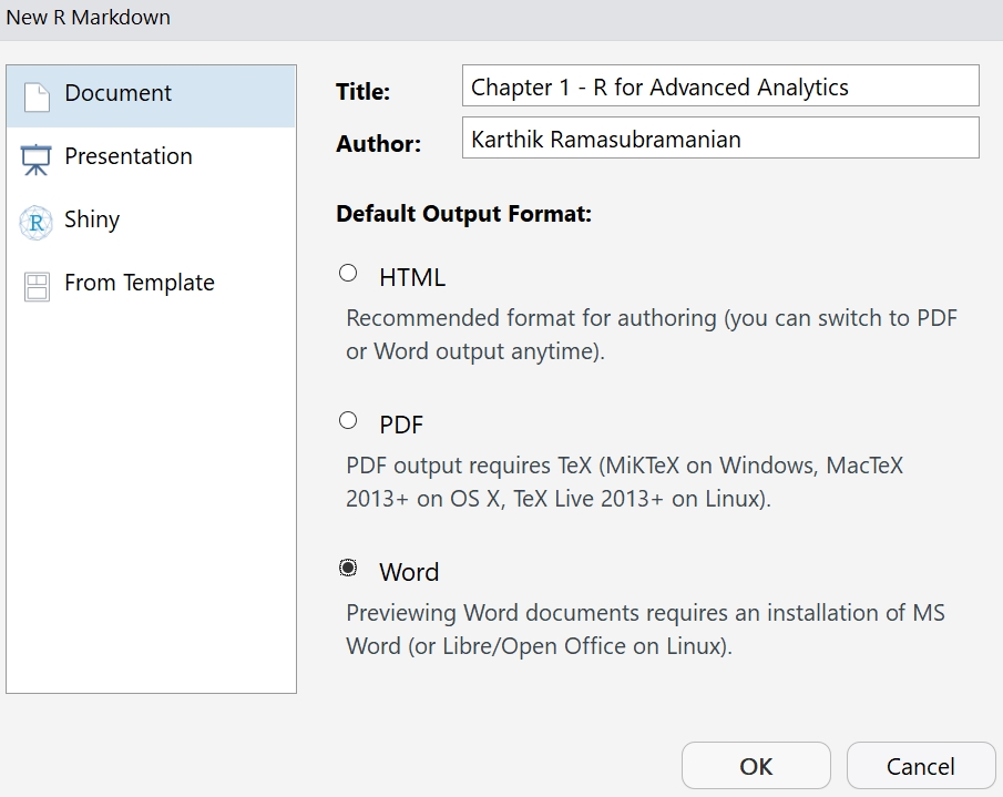
Figure 1.13: Creating a new R Markdown file in Rstudio
Now, use the read.csv() method to read the bank-full.csv file:

Figure 1.14: Using the read.csv method to read the data
Finally, print the summary into a word file using the summary method:

Figure 1.15: Final output after using the summary method
Activity 2: Create a List of Two Matrices and Access the Values
Create two matrices of size 10 x 4 and 4 x 5 by randomly generated numbers from a binomial distribution (use rbinom method). Call the matrix mat_A and mat_B, respectively:
mat_A <- matrix(rbinom(n = 40, size = 100, prob = 0.4),nrow = 10, ncol=4)
mat_B <- matrix(rbinom(n = 20, size = 100, prob = 0.4),nrow = 4, ncol=5)
Now, store the two matrices in a list:
list_of_matrices <- list(mat_A = mat_A, mat_B =mat_B)
Using the list, access the row 4 and column 2 of mat_A and store it in variable A, and access row 2 and column 1 of mat_B and store it in variable B:
A <- list_of_matrices[["mat_A"]][4,2]
B <- list_of_matrices[["mat_B"]][2,1]
Multiply the A and B matrices and subtract from row 2 and column 1 of mat_A:
list_of_matrices[["mat_A"]][2,1] - (A*B)
The output is as follows:
## [1] -1554
Activity 3: Create a DataFrame with Five Summary Statistics for All Numeric Variables from Bank Data Using dplyr and tidyr
Import the dplyr and tidyr packages in the system:
library(dplyr)
library(tidyr)
Warning: package 'tidyr' was built under R version 3.2.5
Create the df DataFrame and import the file into it:
df <- tbl_df(df_bank_detail)
Extract all numeric variables from bank data using select(), and compute min, 1st quartile, 3rd quartile, median, mean, max, and standard deviation using the summarise_all() method:
df_wide <- df %>%
  select(age, balance, duration, pdays) %>%
  summarise_all(funs(min = min,
                      q25 = quantile(., 0.25),
                      median = median,
                      q75 = quantile(., 0.75),
                      max = max,
                      mean = mean,
                      sd = sd))
The result is a wide data frame. 4 variable, 7 measures:
dim(df_wide)
## [1]  1 28
Store the result in a DataFrame of wide format named df_wide, reshape it using the tidyr functions, and, finally, convert the wide format to deep, use the gather, separate, and spread functions of the tidyr package:
df_stats_tidy <- df_wide %>% gather(stat, val) %>%
  separate(stat, into = c("var", "stat"), sep = "_") %>%
  spread(stat, val) %>%
  select(var,min, q25, median, q75, max, mean, sd) # reorder columns
print(df_stats_tidy)
The output is as follows:
## # A tibble: 4 x 8
##        var   min   q25 median   q75    max       mean         sd
## *    <chr> <dbl> <dbl>  <dbl> <dbl>  <dbl>      <dbl>      <dbl>
## 1      age    18    33     39    48     95   40.93621   10.61876
## 2  balance -8019    72    448  1428 102127 1362.27206 3044.76583
## 3 duration     0   103    180   319   4918  258.16308  257.52781
## 4    pdays    -1    -1     -1    -1    871   40.19783  100.12875


