Node classification – predicting student interests

In this section, we’ll implement a GCN to predict student interests based on their features and connections in the social network. This task demonstrates how GNNs can leverage both node attributes and network structure to make predictions about individual nodes.

Let’s start by defining our GCN model:

class GCN(torch.nn.Module):
    def __init__(self, in_channels, hidden_channels, out_channels):
        super().__init__()
        self.conv1 = GCNConv(in_channels, hidden_channels)
        self.conv2 = GCNConv(hidden_channels, out_channels)
    def forward(self, x, edge_index):
        x = self.conv1(x, edge_index).relu()
        x = self.conv2(x, edge_index)
        return x
# Initialize the model
model = GCN(in_channels=num_features,
            hidden_channels=16,
            out_channels=num_classes)

As you can see, our GCN model consists of two graph convolutional layers. The first layer takes the input features and produces hidden representations, while the second layer produces the final class predictions.

Now, let’s train the model. You can view the complete code at https://github.com/PacktPublishing/Applied-Deep-Learning-on-Graphs. Let’s break down the training process here:

1. We define an optimizer (Adam) and a loss function (CrossEntropyLoss) for training our model:

   optimizer = torch.optim.Adam(model.parameters(), lr=0.01)
   criterion = torch.nn.CrossEntropyLoss()

2. The train() function performs one step of training:

   def train():
       model.train()
       optimizer.zero_grad()
       out = model(data.x, data.edge_index)
       loss = criterion(out, data.y)
       loss.backward()
       optimizer.step()
       return loss

   • It sets the model to training mode.
   • It computes the forward pass of the model.
   • It calculates the loss between predictions and true labels.
   • It performs backpropagation and updates the model parameters.
3. The test() function evaluates the model’s performance:

   def test():
       model.eval()
       out = model(data.x, data.edge_index)
       pred = out.argmax(dim=1)
       correct = (pred == data.y).sum()
       acc = int(correct) / int(data.num_nodes)
       return acc

   • It sets the model to evaluation mode.
   • It computes the forward pass.
   • It calculates the accuracy of predictions.
4. We train the model for 200 epochs, printing the loss and accuracy every 10 epochs:

   for epoch in range(200):
       loss = train()
       if epoch % 10 == 0:
           acc = test()
           print(f'Epoch: {epoch:03d}, Loss: {loss:.4f}, \
                 Accuracy: {acc:.4f}')

5. Finally, we evaluate the model one last time to get the final accuracy:

   final_acc = test()
   print(f"Final Accuracy: {final_acc:.4f}")

To visualize how well our model is performing, let’s create a function to plot the predicted versus true interest groups:

def visualize_predictions(model, data):
    model.eval()
    out = model(data.x, data.edge_index)
    pred = out.argmax(dim=1)
    plt.figure(figsize=(10, 5))
    plt.subplot(121)
    plt.title("True Interests")
    plt.scatter(
        data.x[:, 0], data.x[:, 1], c=data.y, cmap='viridis')
    plt.colorbar()
    plt.subplot(122)
    plt.title("Predicted Interests")
    plt.scatter(
        data.x[:, 0], data.x[:, 1], c=pred, cmap='viridis')
    plt.colorbar()
    plt.tight_layout()
    plt.show()
visualize_predictions(model, data)

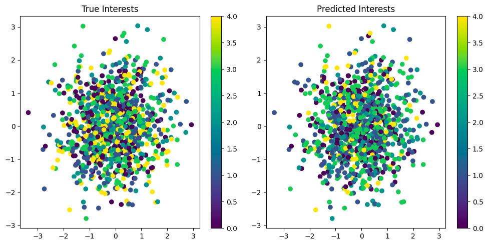
This function creates two scatter plots: one showing the true interest groups and another showing the predicted interest groups.

Figure 7.1: Model performance: true versus predicted interests

In Figure 7.1, each point represents a student, positioned based on their first two features. The visualization consists of two scatter plots labeled True Interests and Predicted Interests. Each point in these plots represents one of the students. The colors in both plots, ranging from purple (0.0) to yellow (4.0), indicate different interest groups. The left plot shows the actual or “true” interest groups of the students, while the right plot displays the model’s predictions of these interest groups. The similarity between the distributions conveys the effectiveness of graph learning techniques in such predictions.

In a real-world application, this node classification task could be used to predict student interests based on their profile information and social connections. This could be valuable for personalized content recommendations, targeted advertising, or improving student engagement in university activities.

Remember that while our synthetic dataset provides a clean example, real-world data often requires more preprocessing, handling of missing values, and careful consideration of privacy and ethical concerns when working with personal data.

Another aspect of graph learning is the task of link prediction. This comes up in a lot of real-world scenarios, especially ones where we are trying to predict certain connections.