Evaluating a model

Once the model has been trained, it is important to evaluate it. In this recipe, we will provide a few insights about a few typical metrics for both classification and regression, before evaluating our model on the test set.

Getting ready

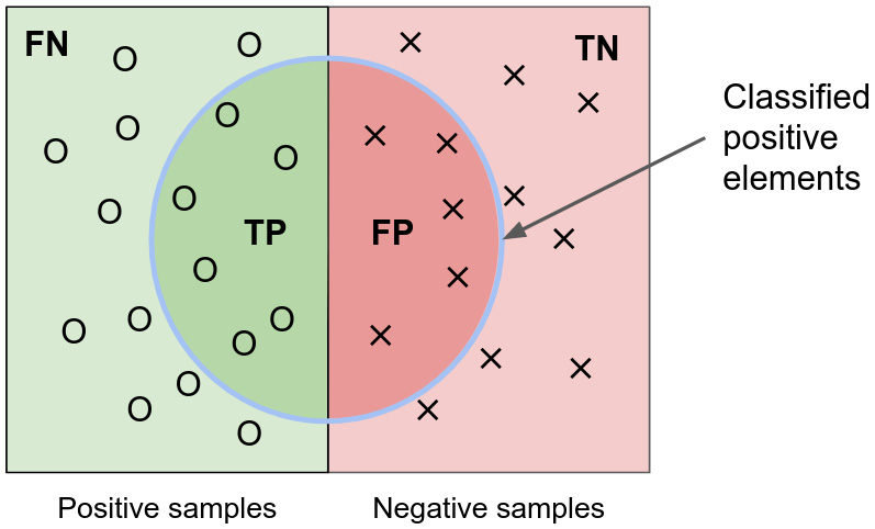
Many evaluation metrics exist. If we think about predicting a binary classification and take a step back, there are only four cases:

• False positive (FP): Positive prediction, negative ground truth
• True positive (TP): Positive prediction, positive ground truth
• True negative (TN): Negative prediction, negative ground truth
• False negative (FN): Negative prediction, positive ground truth:

Figure 2.6 – Representation of false positive, true positive, true negative, and false negative

Based on this, we can define a wide range of evaluation metrics.

One of the most common metrics is accuracy, which is the ratio of good predictions. The definition of accuracy is as follows:

Note

Although very common, the accuracy may be misleading, especially for imbalanced labels. For example, let’s assume an extreme case where 99% of Titanic passengers survived, and we have a model that predicts that every passenger survived. Our model would have a 99% accuracy but would be wrong for 100% of passengers who did not survive.

There are several other very common metrics, such as precision, recall, and the F1 score.

Precision is most suited when you’re trying to maximize the true positives and minimize the false positives – for example, making sure you detect only surviving passengers:

Recall is most suited when you’re trying to maximize the true positives and minimize the false negatives – for example, making sure you don’t miss any surviving passengers:

The F1 score is just a combination of the precision and recall metrics as a harmonic mean:

Another useful classification evaluation metric is the Receiver Operating Characteristic Area Under Curve (ROC AUC) score.

All these metrics behave similarly: when there are values between 0 and 1, the higher the value, the better the model. Some are also more robust to imbalanced labels, especially the F1 score and ROC AUC.

For regression tasks, the most used metrics are the mean squared error (MSE) and the R2 score.

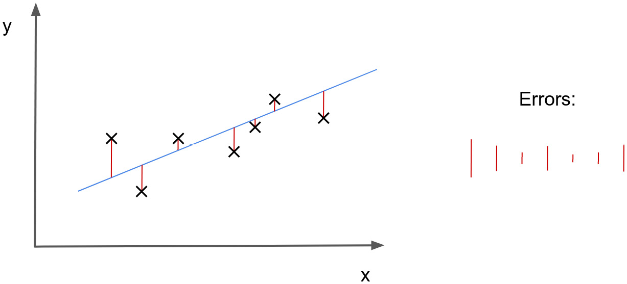
The MSE is the averaged square difference between the predictions and the ground truth:

Here, m is the number of samples, ŷ is the predictions, and y is the ground truth:

Figure 2.7 – Visualization of the errors for a regression task

In terms of the R2 score, it is a metric that can be negative and is defined as follows:

Note

While the R2 score is a typical evaluation metric (the closer to 1, the better), the MSE is more typical of a loss function (the closer to 0, the better).

How to do it…

Assuming our chosen evaluation metric here is accuracy, a very simple way to evaluate our model is to use the accuracy_score() function:

from sklearn.metrics import accuracy_score
# Compute the accuracy on test of our model
print('accuracy on test set:', accuracy_score(y_pred,
    y_test))

This outputs the following:

accuracy on test set: 0.7877094972067039

Here, the accuracy_score() function provides an accuracy of 78.77%, meaning about 79% of our model’s predictions are right.

See also

Here is a list of the available metrics in scikit-learn: https://scikit-learn.org/stable/modules/classes.html#module-sklearn.metrics.