Building a polynomial regressor

One of the main constraints of a linear regression model is the fact that it tries to fit a linear function to the input data. The polynomial regression model overcomes this issue by allowing the function to be a polynomial, thereby increasing the accuracy of the model.

Getting ready

Polynomial models should be applied where the relationship between response and explanatory variables is curvilinear. Sometimes, polynomial models can also be used to model a non-linear relationship in a small range of explanatory variable. A polynomial quadratic (squared) or cubic (cubed) term converts a linear regression model into a polynomial curve. However, since it is the explanatory variable that is squared or cubed and not the beta coefficient, it is still considered as a linear model. This makes it a simple and easy way to model curves, without needing to create big non-linear models. Let's consider the following diagram:

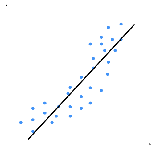
We can see that there is a natural curve to the pattern of data points. This linear model is unable to capture this. Let's see what a polynomial model would look like:

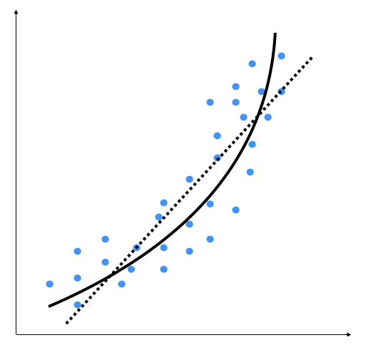
The dotted line represents the linear regression model, and the solid line represents the polynomial regression model. The curviness of this model is controlled by the degree of the polynomial. As the curviness of the model increases, it gets more accurate. However, curviness adds complexity to the model as well, making it slower. This is a trade-off: you have to decide how accurate you want your model to be given the computational constraints.

How to do it...

Let's see how to build a polynomial regressor in Python:

In this example, we will only deal with second-degree parabolic regression. Now, we'll show how to model data with a polynomial. We measured the temperature for a few hours of the day. We want to know the temperature trend even at times of the day when we did not measure it. Those times are, however, between the initial time and the final time at which our measurements took place:

import numpy as np

Time = np.array([6, 8, 11, 14, 16, 18, 19])
Temp = np.array([4, 7, 10, 12, 11.5, 9, 7])

Now, we will show the temperature at a few points during the day:

import matplotlib.pyplot as plt
plt.figure()
plt.plot(Time, Temp, 'bo')
plt.xlabel("Time")
plt.ylabel("Temp")
plt.title('Temperature versus time')
plt.show()

The following graph is produced:

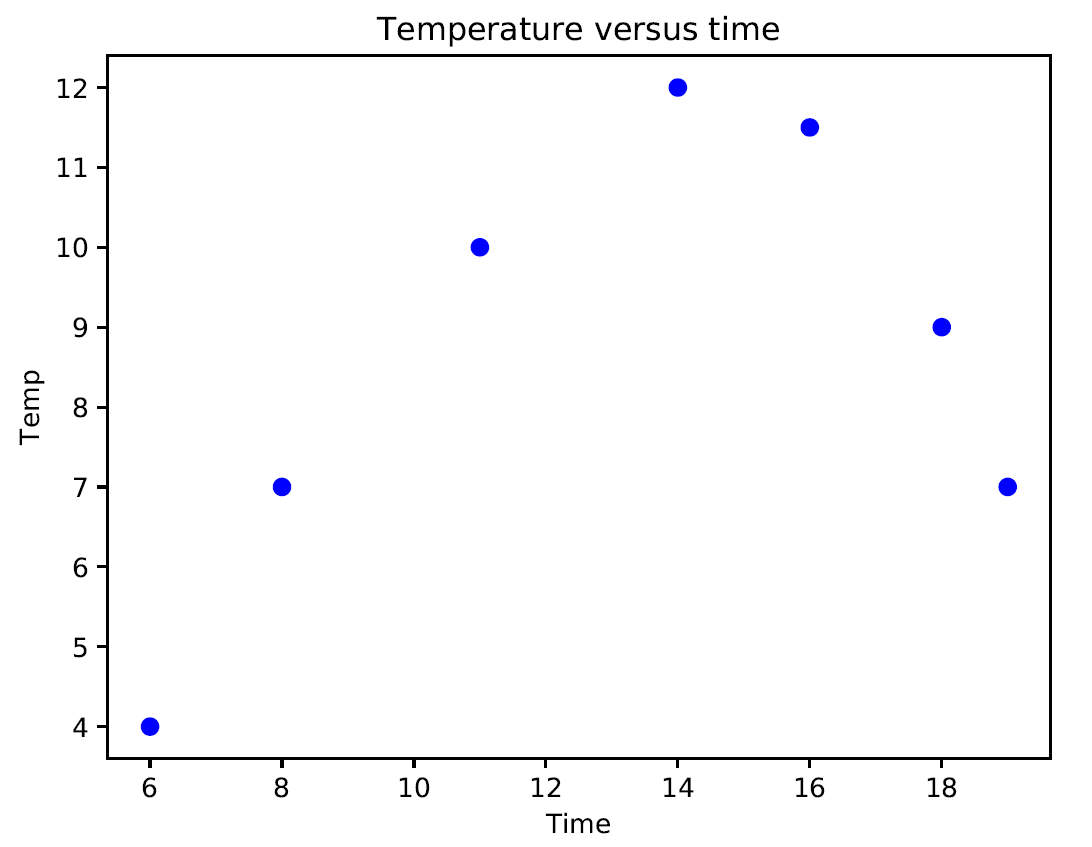
If we analyze the graph, it is possible to note a curvilinear pattern of the data that can be modeled through a second-degree polynomial such as the following equation:

The unknown coefficients, β₀, β₁, and β₂, are estimated by decreasing the value of the sum of the squares. This is obtained by minimizing the deviations of the data from the model to its lowest value (least squares fit).

Let's calculate the polynomial coefficients:

beta = np.polyfit(Time, Temp, 2)

The numpy.polyfit() function returns the coefficients for a polynomial of degree n (given by us) that is the best fit for the data. The coefficients returned by the function are in descending powers (highest power first), and their length is n+1 if n is the degree of the polynomial.

After creating the model, let's verify that it actually fits our data. To do this, use the model to evaluate the polynomial at uniformly spaced times. To evaluate the model at the specified points, we can use the poly1d() function. This function returns the value of a polynomial of degree n evaluated at the points provided by us. The input argument is a vector of length n+1 whose elements are the coefficients in descending powers of the polynomial to be evaluated:

p = np.poly1d(beta)

As you can see in the upcoming graph, this is close to the output value. If we want it to get closer, we need to increase the degree of the polynomial.

Now we can plot the original data and the model on the same plot:

xp = np.linspace(6, 19, 100)
plt.figure()
plt.plot(Time, Temp, 'bo', xp, p(xp), '-')
plt.show()

The following graph is printed:

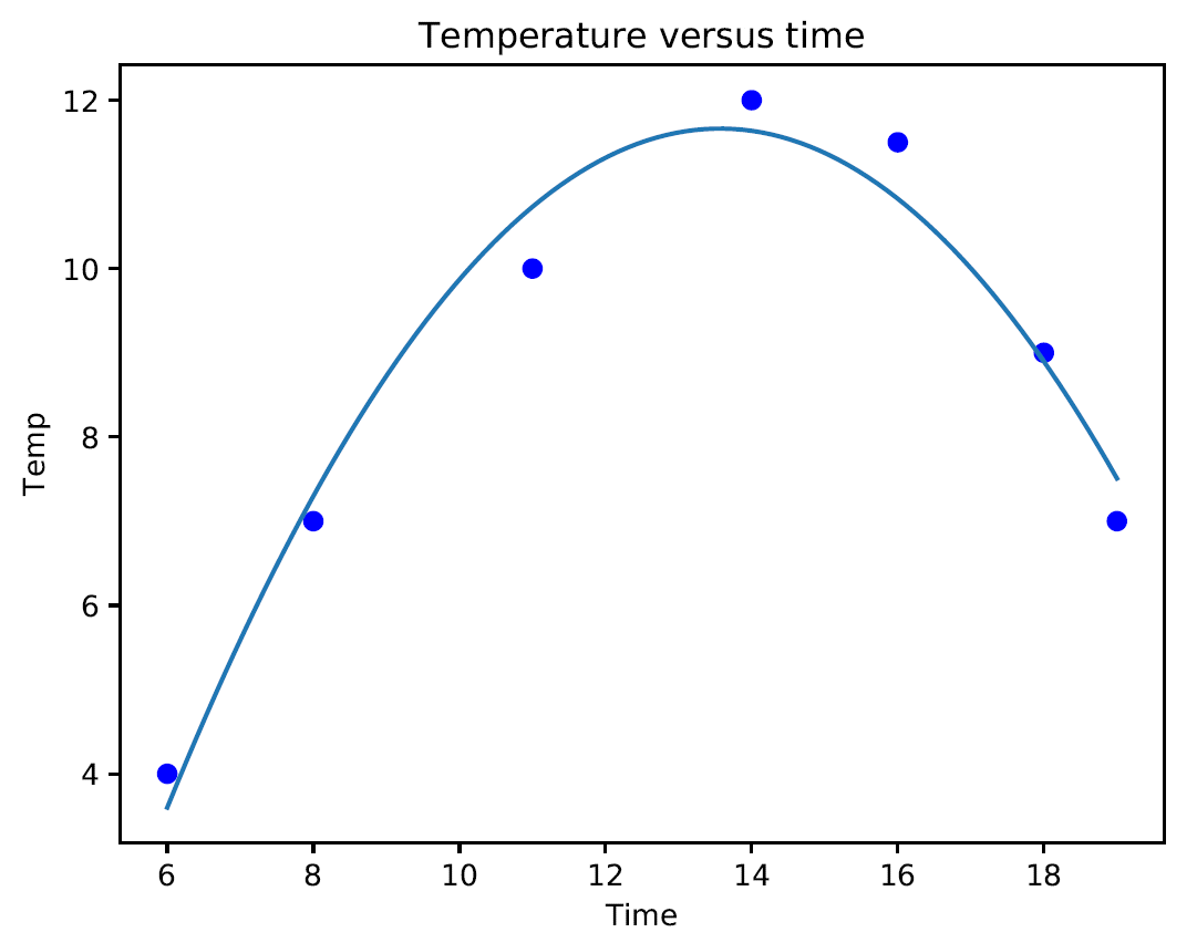
If we analyze the graph, we can see that the curve fits our data sufficiently. This model fits the data to a greater extent than a simple linear regression model. In regression analysis, it's important to keep the order of the model as low as possible. In the first analysis, we keep the model as a first order polynomial. If this is not satisfactory, then a second-order polynomial is tried. The use of higher-order polynomials can lead to incorrect evaluations.

How it works...

Polynomial regression should be used when linear regression is not good enough. With polynomial regression, we approached a model in which some predictors appear in degrees equal to or greater than two to fit the data with a curved line. Polynomial regression is usually used when the relationship between variables looks curved.

There's more...

At what degree of the polynomial must we stop? It depends on the degree of precision we are looking for. The higher the degree of the polynomial, the greater the precision of the model, but the more difficult it is to calculate. In addition, it is necessary to verify the significance of the coefficients that are found, but let's get to it right away.