In this section, we will look at some examples of how ML is used, and with each example, we'll speculate about the type of data, learning style, and ML algorithm used. I hope that by the end of this section, you will be inspired by what is possible with ML and gain some appreciation for the types of data, algorithms, and learning styles that exist.
A brief tour of ML algorithms
Netflix – making recommendations
No ML book is complete without mentioning recommendation engines—probably one of the most well known applications of ML. In part, this is thanks to the publicity gained when Netflix announced a $1 million competition for movie rating predictions, also known as recommendations. Add to this Amazon's commercial success in making use of it.
The goal of recommendation engines is to predict the likelihood of someone wanting a particular product or service. In the context of Netflix, this would mean recommending movies or TV shows to its users.
One intuitive way of making recommendations is to try and mimic the real world, where a person is likely to seek recommendations from like-minded people. What constitutes likeness is dependent on the domain. For example, you are most likely to have one group of friends that you would ask for restaurant recommendations and another group of friends for movie recommendations. What determines these groups is how similar their tastes are to your own taste for that particular domain. We can replicate this using the (user-based) Collaborative Filtering (CF) algorithm. This algorithm achieves this by finding the distance between each user and then using these distances as a similarity metric to infer predictions on movies for a particular user; that is, those that are more similar will contribute more to the prediction than those that have different preferences. Let's have a look at what form the data might take from Netflix:
| User | Movie | Rating |
| 0: Jo | A: Monsters Inc | 5 |
| B: The Bourne Identity | 2 | |
| C: The Martian | 2 | |
| D: Blade Runner | 1 | |
| 1: Sam | C: The Martian | 4 |
| D: Blade Runner | 4 | |
| E: The Matrix | 4 | |
| F: Inception | 5 | |
| 2: Chris | B: The Bourne Identity | 4 |
| C: The Martian | 5 | |
| D: Blade Runner | 5 | |
| F: Inception | 4 |
For each example, we have a user, a movie, and an assigned rating. To find the similarity between each user, we can first calculate the Euclidean distance of the shared movies between each pair of users. The Euclidean distance gives us larger values for users who are most dissimilar; we invert this by dividing 1 by this distance to give us a result, where 1 represents perfect matches and 0 means the users are most dissimilar. The following is the formula for Euclidean distance and the function used to calculate similarities between two users:

func calcSimilarity(userRatingsA: [String:Float], userRatingsB:[String:Float]) -> Float{
  var distance = userRatingsA.map( { (movieRating) -> Float in
    if userRatingsB[movieRating.key] == nil{
      return 0
    }
    let diff = movieRating.value - (userRatingsB[movieRating.key] ?? 0)
    return diff * diff
  }).reduce(0) { (prev, curr) -> Float in
    return prev + curr
  }.squareRoot()
  return 1 / (1 + distance)
}
To make this more concrete, let's walk through how we can find the most similar user for Sam, who has rated the following movies: ["The Martian" : 4, "Blade Runner" : 4, "The Matrix" : 4, "Inception" : 5]. Let's now calculate the similarity between Sam and Jo and then between Sam and Chris.
Sam and Jo
Jo has rated the movies ["Monsters Inc." : 5, "The Bourne Identity" : 2, "The Martian" : 2, "Blade Runner" : 1]; by calculating the similarity of intersection of the two sets of ratings for each user, we get a value of 0.22.
Sam and Chris
Similar to the previous ones, but now, by calculating the similarity using the movie ratings from Chris (["The Bourne Identity" : 4, "The Martian" : 5, "Blade Runner" : 5, "Inception" : 4]), we get a value of 0.37.
Through manual inspection, we can see that Chris is more similar to Sam than Jo is, and our similarity rating shows this by giving Chris a higher value than Jo.
To help illustrate why this works, let's project the ratings of each user onto a chart as shown in the following graph:
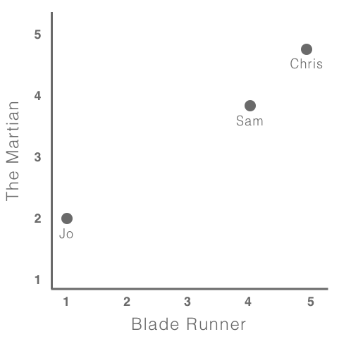
The preceding graph shows the users plotted in a preference space; the closer two users are in this preference space, the more similar their preferences are. Here, we are just showing two axes, but, as seen in the preceding table, this extends to multiple dimensions.
We can now use these similarities as weights that contribute to predicting the rating a particular user would give to a particular movie. Then, using these predictions, we can recommend some movies that a user is likely to want to watch.
The preceding approach is a type of clustering algorithm that falls under unsupervised learning, a learning style where examples have no associated label and the job of the ML algorithm is to find patterns within the data. Other common unsupervised learning algorithms include the Apriori algorithm (basket analysis) and K-means.
Recommendations are applicable anytime when there is an abundance of information that can benefit from being filtered and ranked before being presented to the user. Having recommendations performed on the device offers many benefits, such as being able to incorporate the context of the user when filtering and ranking the results.
Shadow draw – real-time user guidance for freehand drawing
To highlight the synergies between man and machine, AI is sometimes referred to as Augmented Intelligence (AI), putting the emphasis on the system to augment our abilities rather than replacing us altogether.
One area that is becoming increasingly popular—and of particular interest to myself—is assisted creation systems, an area that sits at the intersection of the fields of human-computer interaction (HCI) and ML. These are systems created to assist in some creative tasks such as drawing, writing, video, and music.
The example we will discuss in this section is shadow draw, a research project undertaken at Microsoft in 2011 by Y.J. Lee, L. Zitnick, and M. Cohen. Shadow draw is a system that assists the user in drawing by matching and aligning a reference image from an existing dataset of objects and then lightly rendering shadows in the background to be used as guidelines for the user. For example, if the user is predicted to be drawing a bicycle, then the system would render guidelines under the user's pen to assist them in drawing the object, as illustrated in this diagram:
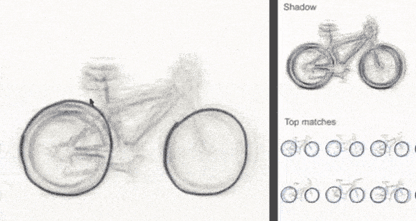
As we did before, let's walk through how we might approach this, focusing specifically on classifying the sketch; that is, we'll predict what object the user is drawing. This will give us the opportunity to see new types of data, algorithms, and applications of ML.
The dataset used in this project consisted of 30,000 natural images collected from the internet via 40 category queries such as face, car, and bicycle, with each category stored in its own directory; the following diagram shows some examples of these images:

After obtaining the raw data, the next step, and typical of any ML project, is to perform data preprocessing and feature engineering. The following diagram shows the preprocessing steps, which consist of:
- Rescaling each image
- Desaturating (turning black and white)
- Edge detection
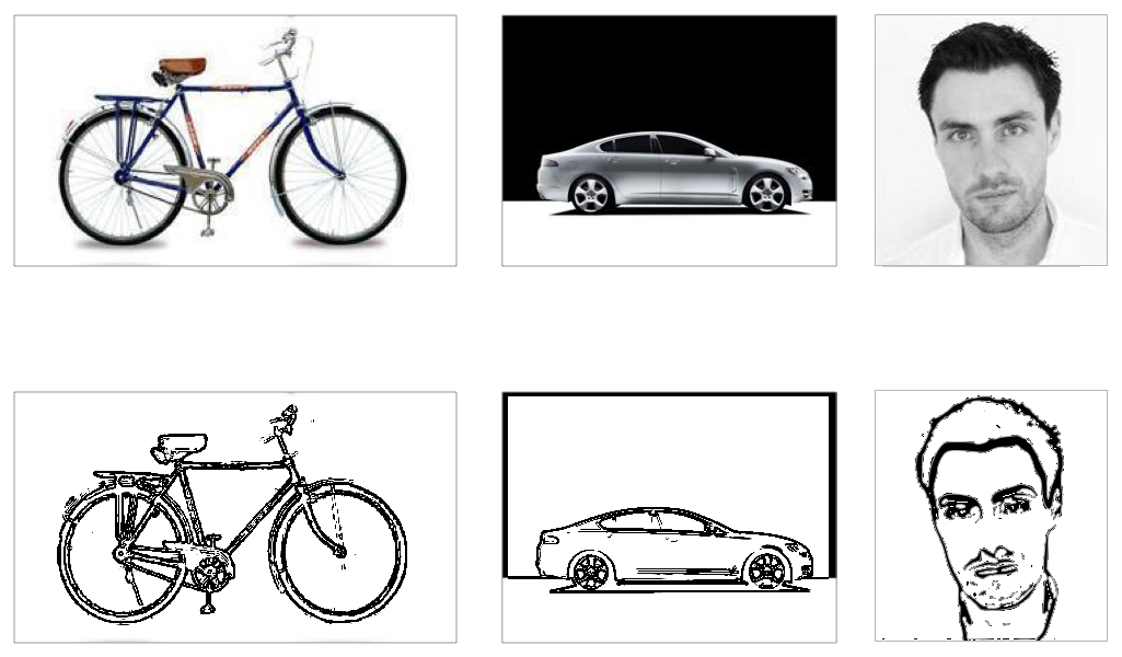
Our next step is to abstract our data into something more meaningful and useful for our ML algorithm to work with; this is known as feature engineering, and is a critical step in a typical ML workflow.
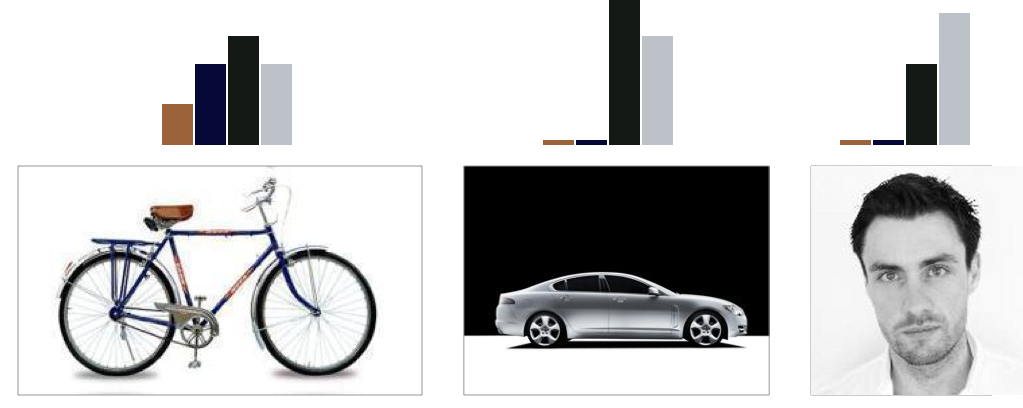
One approach, and the approach we will describe, is creating something known as a visual bag of words. This is essentially a histogram of features (visual words) used to describe each image, and collectively to describe each category. What constitutes a feature is dependent on the data and ML algorithm; for example, we can extract and count the colors of each image, where the colors become our features and collectively describe our image, as shown in the following diagram:
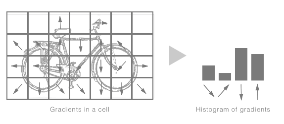
But because we are dealing with sketches, we want something fairly coarse—something that can capture the general strokes directions that will encapsulate the general structure of the image. For example, if we were to describe a square and a circle, the square would consist of horizontal and vertical strokes, while the circle would consist mostly of diagonal strokes. To extract these features, we can use a computer vision algorithm called histogram of oriented gradients (HOG); after processing an image you are returned a histogram of gradient orientations in localized portions of the image. Exactly what we want! To help illustrate the concept, this process is summarized for a single image here:
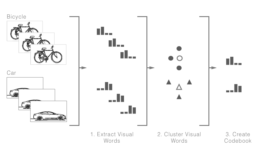
After processing all the images in our dataset, our next step is to find a histogram (or histograms) that can be used to identify each category; we can use an unsupervised learning clustering technique called K-means, where each category histogram is the centroid for that cluster. The following diagram describes this process; we first extract features for each image and then cluster these using K-means, where the distance is calculated using the histogram of gradients. Once our images have been clustered into their groups, we extract the center (mean) histogram of each of these groups to act as our category descriptor:
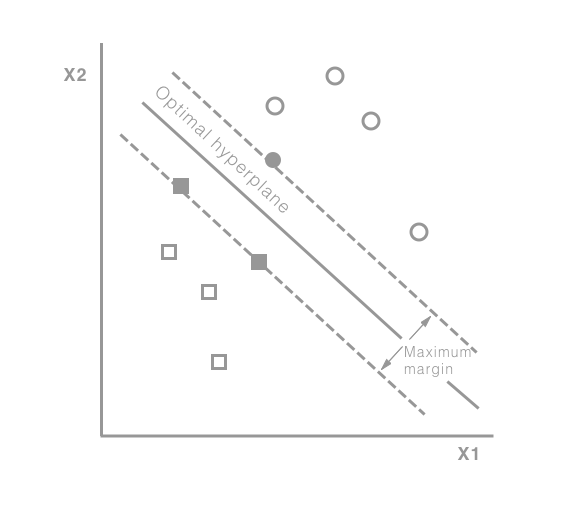
Once we have obtained a histogram for each category (codebook), we can train a classifier using each image's extracted features (visual words) and the associated category (label). One popular and effective classifier is support vector machines (SVM). What SVM tries to find is a hyperplane that best separates the categories; here, best refers to a plane that has the largest distance between each of the category members. The term hyper is used because it transforms the vectors into high-dimensional space such that the categories can be separated with a linear plane (plane because we are working within a space). The following diagram shows how this may look for two categories in a two-dimensional space:
With our model now trained, we can perform real-time classification on the image as the user is drawing, thus allowing us to assist the user by providing them with guidelines for the object they are wanting to draw (or at least, mention the object we predicted them to be drawing). Perfectly suited for touch interfaces such as your iPhone or iPad! This assists not just in drawing applications, but anytime where an input is required by the user, such as image-based searching or note taking.
In this example, we showed how feature engineering and unsupervised learning are used to augment data, making it easier for our model to sufficiently perform classification using the supervised learning algorithm SVM. Prior to deep neural networks, feature engineering was a critical step in ML and sometimes a limiting factor for these reasons:
- It required special skills and sometimes domain expertise
- It was at the mercy of a human being able to find and extract meaningful features
- It required that the features extracted would generalize across the population, that is, be expressive enough to be applied to all examples
In the next example, we introduce a type of neural network called a convolutional neural network (CNN or ConvNet), which takes care of a lot of the feature engineering itself.
Shutterstock – image search based on composition
Over the past 10 years, we have seen an explosive growth in visual content created and consumed on the Web, but before the success of CNNs, images were found by performing simple keyword searches on the tags assigned manually. All this changed around 2012, when A. Krizhevsky, I. Sutskever, and G. E. Hinton published their paper ImageNet Classification with Deep Convolutional Networks. The paper described their architecture used to win the 2012 ImageNet Large-Scale Visual Recognition Challenge (ILSVRC). It's a competition like the Olympics of computer vision, where teams compete across a range of CV tasks such as classification, detection, and object localization. And that was the first year a CNN gained the top position with a test error rate of 15.4% (the next best entry achieved an test error rate of 26.2%). Ever since then, CNNs have become the de facto approach for computer vision tasks, including becoming the new approach for performing visual search. Most likely, it has been adopted by the likes of Google, Facebook, and Pinterest, making it easier than ever to find that right image.
Recently, (October 2017), Shutterstock announced one of the more novel uses of CNNs, where they introduced the ability for their users to search for not only multiple items in an image, but also the composition of those items. The following screenshot shows an example search for a kitten and a computer, with the kitten on the left of the computer:

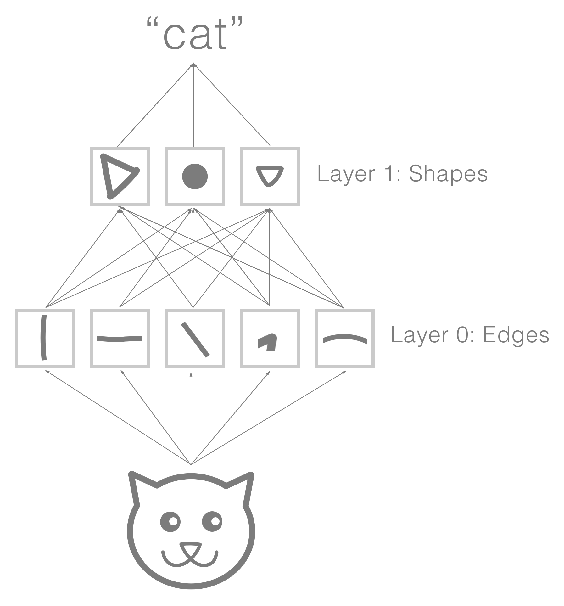
So what are CNNs? As previously mentioned, CNNs are a type of neural network that are well suited for visual content due to their ability to retain spatial information. They are somewhat similar to the previous example, where we explicitly define a filter to extract localized features from the image. A CNN performs a similar operation, but unlike our previous example, filters are not explicitly defined. They are learned through training, and they are not confined to a single layer but rather build with many layers. Each layer builds upon the previous one and each becomes increasingly more abstract (abstract here means a higher-order representation, that is, from pixels to shapes) in what it represents.
To help illustrate this, the following diagram visualizes how a network might build up its understanding of a cat. The first layer's filters extract simple features, such as edges and corners. The next layer builds on top of these with its own filters, resulting in higher-level concepts being extracted, such as shapes or parts of the cat. These high-level concepts are then combined for classification purposes:
To train the model, we feed the network examples using images as inputs and labels as the expected outputs. Given enough examples, the model will build an internal representation for each label, which can be sufficiently used for classification; this, of course, is a type of supervised learning.
Our last task is to find the location of the item or items; to achieve this, we can inspect the weights of the network to find out which pixels activated a particular class, and then create a bounding box around the inputs with the largest weights.
We have now identified the items and their locations within the image. With this information, we can preprocess our repository of images and cache it as metadata to make it accessible via search queries. We will revisit this idea later in the book when you will get a chance to implement a version of this to assist the user in finding images in their photo album.
In this section, we saw how ML can be used to improve user experience and briefly introduced the intuition behind CNNs, a neural network well suited for visual contexts, where retaining proximity of features and building higher levels of abstraction is important. In the next section, we will continue our exploration of ML applications by introducing another example that improves the user experience and a new type of neural network that is well suited for sequential data such as text.
iOS keyboard prediction – next letter prediction
Quoting usability expert Jared Spool, Good design, when done well, should be invisible. This holds true for ML as well. The application of ML need not be apparent to the user and sometimes (more often than not) more subtle uses of ML can prove just as impactful.
A good example of this is an iOS feature called dynamic target resizing; it is working every time you type on an iOS keyboard, where it actively tries to predict what word you're trying to type:
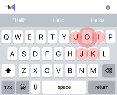
Using this prediction, the iOS keyboard dynamically changes the touch area of a key (here illustrated by the red circles) that is the most likely character based on what has already been typed before it.
For example, in the preceding diagram, the user has entered "Hell"; now it would be reasonable to assume that the most likely next character the user wants to tap is "o". This is intuitive given our knowledge of the English language, but how do we teach a machine to know this?
This is where recurrent neural networks (RNNs) come in; it's a type of neural network that persists state over time. You can think of this persisted state as a form of memory, making RNNs suitable for sequential data such as text (any data where the inputs and outputs are dependent on each other). This state is created by using a feedback loop from the output of the cell, as shown in the following diagram:
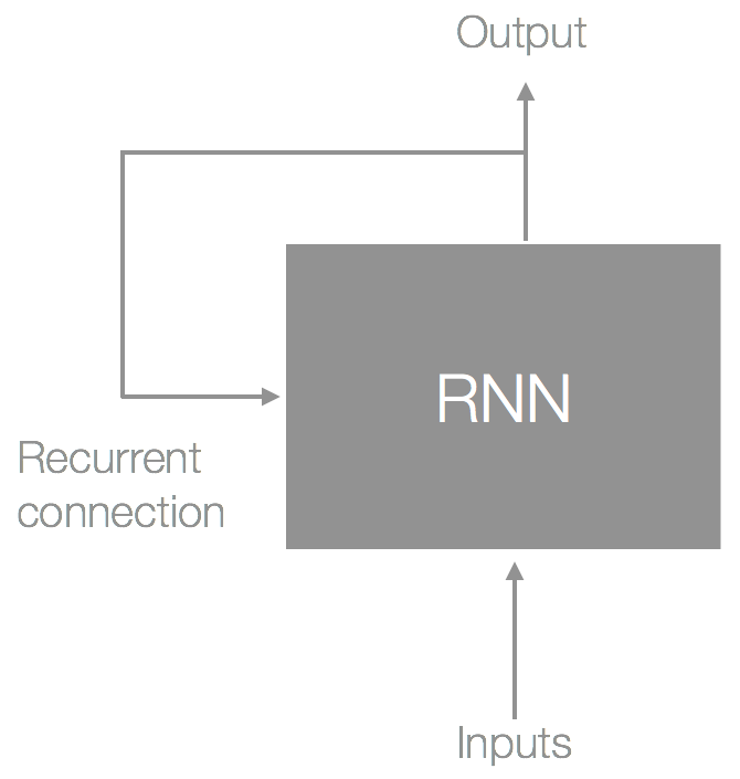
The preceding diagram shows a single RNN cell. If we unroll this over time, we would get something that looks like the following:
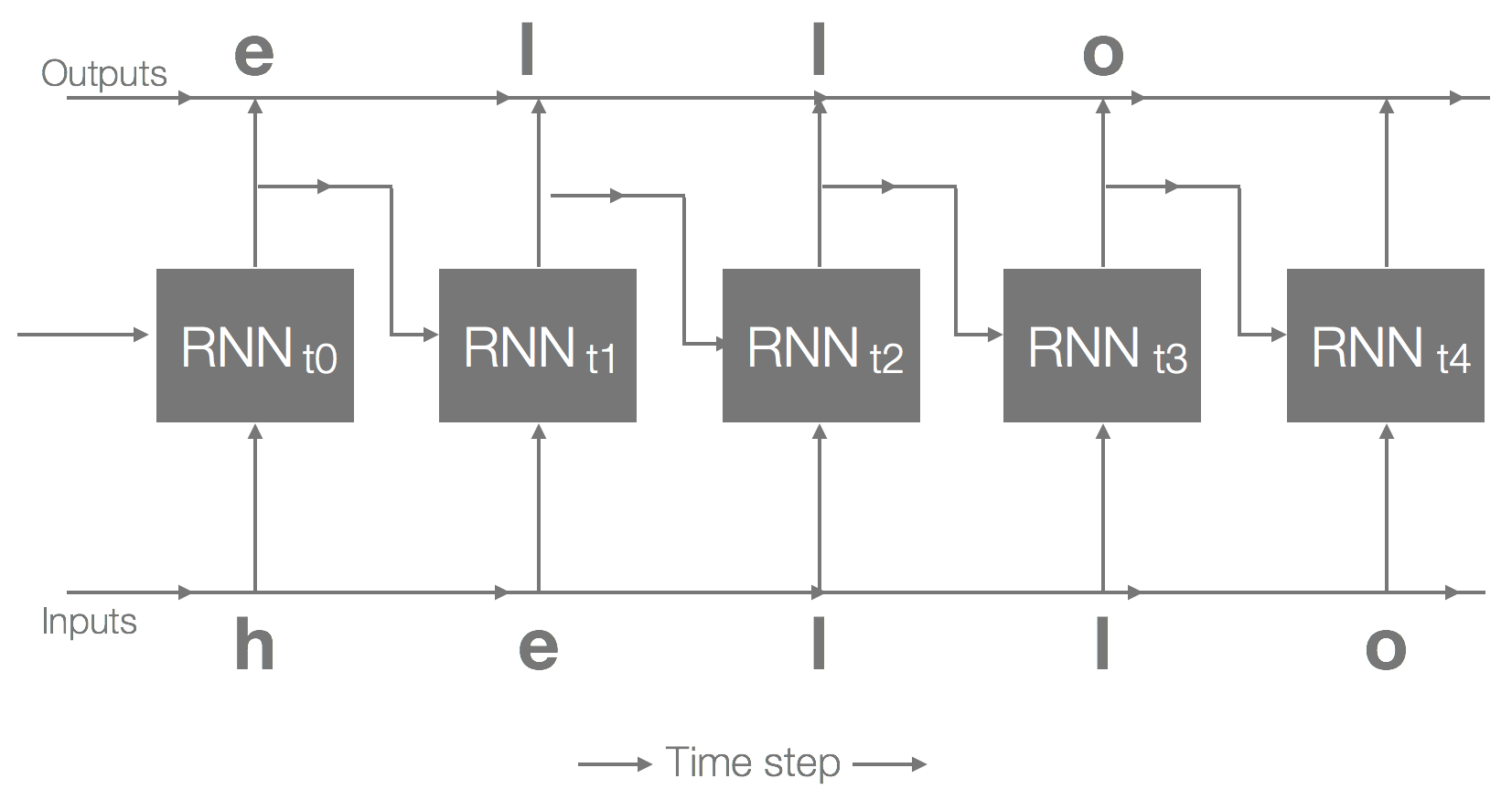
Using hello as our example, the preceding diagram shows an unrolled RNN over five time steps; at each time step, the RNN predicts the next likely character. This prediction is determined by its internal representation of the language (from training) and subsequent inputs. This internal representation is built by training it on samples of text where the output is using the inputs but at the next time step (as illustrated earlier). Once trained, the inference follows a similar path, except that we feed to the network the predicted character from the output, to get the next output (to generate the sequence, that is, words).
Neural networks and most ML algorithms require their inputs to be numbers, so we need to convert our characters to numbers, and back again. When dealing with text (characters and words), there are generally two approaches: one-hot encoding and embeddings. Let's quickly cover each of these to get some intuition of how to handle text.
Text (characters and words) is considered categorical, meaning that we cannot use a single number to represent text because there is no inherit relationship between the text and the value; that is, assigning the 10 and cat 20 implies that cat has a greater value than the. Instead, we need to encode them into something where no bias is introduced. One solution to this is encoding them using one-hot encoding, which uses an array of the size of your vocabulary (number of characters in our case), with the index of the specific character set to 1 and the rest set to 0. The following diagram illustrates the encoding process for the corpus "hello":

In the preceding diagram, we show some of the steps required when encoding characters; we start off by splitting the corpus into individual characters (called tokens, and the process is called tokenization). Then we create a set that acts as our vocabulary, and finally we encode this with each character being assigned a vector.
Once our inputs are encoded, we can feed them into our network. Outputs will also be represented in this format, with the most likely character being the index with the greatest value. For example, if 'e' is predicted, then the most likely the output may resemble something like [0.95, 0.2, 0.2, 0.1].
But there are two problems with one-hot encoding. The first is that for a large vocabulary, we end up with a very sparse data structure. This is not only an inefficient use of memory, but also requires additional calculations for training and inference. The second problem, which is more obvious when operating on words, is that we lose any contextual meaning after they have been encoded. For example, if we were to encode the words dog and dogs, we would lose any relationship between these words after encoding.
An alternative, and something that addresses these two problems, is using an embedding. These are generally weights from a trained network that use a dense vector representation for each token, one that preserves some contextual meaning. This book focuses on computer vision tasks, so we won't be going into the details here. Just remember that we need to encode our text (characters) into something our ML algorithm will accept.
We train the model using weak supervision, similar to supervised learning, but inferring the label without it having been explicitly labelled. Once trained, we can predict the next character using multi-class classification, as described earlier.
Over the past couple of years, we have seen the evolution of assistive writing; one example is Google's Smart Reply, which provides an end-to-end method for automatically generating short email responses. Exciting times!
This concludes our brief tour of introducing types of ML problems along with the associated data types, algorithms, and learning style. We have only scratched the surface of each, but as you make your way through this book, you will be introduced to more data types, algorithms, and learning styles.
In the next section, we will take a step back and review the overall workflow for training and inference before wrapping up this chapter.


