Search icon CANCEL
Subscription
0
Cart icon
Your Cart (0 item)
Close icon
You have no products in your basket yet
Arrow left icon
Explore Products
Best Sellers
New Releases
Books
Videos
Audiobooks
Learning Hub
Conferences
Free Learning
Arrow right icon
Arrow up icon
GO TO TOP
Hands-On Java Deep Learning for Computer Vision

You're reading from   Hands-On Java Deep Learning for Computer Vision Implement machine learning and neural network methodologies to perform computer vision-related tasks

Arrow left icon
Product type Paperback
Published in Feb 2019
Publisher Packt
ISBN-13 9781789613964
Length 260 pages
Edition 1st Edition
Languages
Arrow right icon
Author (1):
Arrow left icon
Klevis Ramo Klevis Ramo
Author Profile Icon Klevis Ramo
Klevis Ramo
Arrow right icon
View More author details
Toc

Table of Contents (8) Chapters Close

Preface 1. Introduction to Computer Vision and Training Neural Networks 2. Convolutional Neural Network Architectures FREE CHAPTER 3. Transfer Learning and Deep CNN Architectures 4. Real-Time Object Detection 5. Creating Art with Neural Style Transfer 6. Face Recognition 7. Other Books You May Enjoy

Representing images and outputs

This section mainly focuses on how images are represented on a computer and how to feed this to the neural network. Based on what we've learned so far, neural networks predict only binary classes, where the answer is yes or no, or right or wrong. Consider the example of predicting whether a patient would have heart disease or not. The answer to this is binary in nature—yes or no. We will now learn to train our neural network to predict multiple classes using softmax.

A computer perceives an image as a two-dimensional matrix of numbers. Look at the following diagram:
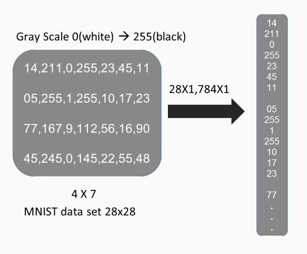
These numbers make little sense to us, but to a computer they mean everything. For a black-and-white image, each of these pixel values depicts the intensity of the light, so zero means white, and as we move closer to the number 255, the pixel gets darker. In this case, we considered an image with the dimensions 4 x 7. Images of the MNIST database are actually 28 x 28 in size. In order to make an image ready for processing, we need to transform it to a one-dimensional vector, which means that a 28 x 28 image will be transformed to 784 x 1 image and a 4 x 7 image to a 28 x 1.

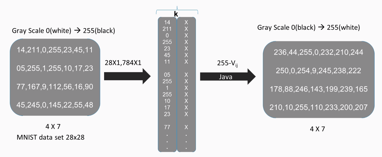
Notice now how this one-dimensional vector is no different from a binary class case. Each of these pixels now is just a feature for a computer vision application. We can, of course, add k-images representations, if we choose a mini-batch gradient descent, which would process k-images in parallel.

When using Java, the values are parameters and their significance is inverse in nature. Here, 0 means black and 255 means white. In order to correctly depict an MNIST dataset image using Java, we need to use the formula, where is the value of the pixel. This happens to be the case with most languages similar to Java:
For colored images, consider an RGB-color JPG, which has a size of 260 x 194 pixels. The computer will see it as a three-dimensional matrix of numbers. Specifically, it will see it as 260 x 194 x 3. Each of the dimensions represents the intensity of the red color, the green color, and the blue color:

So if we take the red example, 0 means the color black, and 255 will be completely red. The same logic applies to the green and the blue colors. We need to transform the three-dimensional matrix to a one-dimensional vector, just as we did previously:
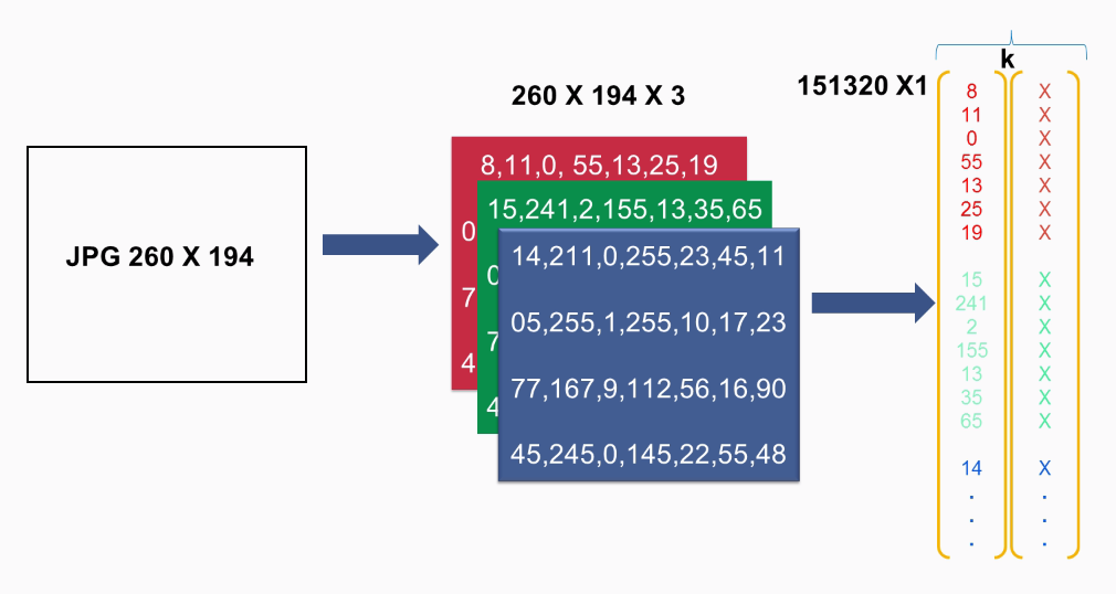
We can also add k-images by choosing mini-batch gradient descent and processing k-images in parallel.

Notice how the number of features dramatically increases for color images, from 784 to 150,000 features. Due to this, the processing time of the image increases drastically, which is where we need to implement techniques to increase the speed of our model.

Multiclass classification

So far, we've seen multiple activation functions, but the one thing that remains constant is the limitation that they can provide only two classes, 0 or 1. Consider the heart disease example:

The neural network predicted 15% not having heart disease and 85% having heart disease, and we set the threshold to 50%. This implies that as soon as one of these percentages exceeds the threshold, we output its index, which would be 0 or 1. In this example, obviously 85% is greater than 50%, so we will output 1, meaning that this person will not have heart disease in the future.

These days, neural networks can actually predict thousands of classes. In the case of ImageNet, we can predict thousands of images. We do this by labeling our images with more than just 0 and 1. Look at the following photos:

Here, we label the photos from 0 to 6 and let the neural network assign each image some percentage. In this case, we consider the maximum, which would be 38%. The neural network will then give us image 4 as the output. Notice how the sum of these percentages will be 100%.

Let us now move into implementing the multiclass classification. Here is what we have seen so far:

This is a neural network containing an activation function in the outer layer. Let us replace this activation function with three nodes, assuming we need to predict three classes instead of two:

Each of these nodes will have a different function, which will be . Thus, we will have , , and , sum up this , and conclude by dividing by the sum of the three values. This step of division is just to make sure that the sum of these percentages will be 100%.

Consider an example where is 5, making equal to 148.4. is 2, which makes equal to 7.4. Similarly, can be set to -1 and will be equal to 0.4. The sum of these values is 156.2. The next step, as discussed, is dividing each of these values by the sum to attain the final percentages.


For class 1, we get 95%, class 2 gives us 4.7%, and class 3 gives us 0.3%.

As logic dictates, the neural network will choose class 1 as the outcome. And since 95% is much greater than 50%, this is what we will choose as a threshold.

Here is what our final neural network looks like:

The weights depicted by the subscript 1 are going to the hidden layer 1, and the weights depicted by the subscript 2 are for the hidden layer 2.

The Z values are the sum of multiplication of the inputs with the weights, which, in this case, is the sum of the multiplication of the activation function with the weights.

In reality, we have another weight called the bias, b, which is added to the older value Z. The following diagram should help you understand this better:

The bias weight is updated in the same way as the v weight.

lock icon The rest of the chapter is locked
Register for a free Packt account to unlock a world of extra content!
A free Packt account unlocks extra newsletters, articles, discounted offers, and much more. Start advancing your knowledge today.
Unlock this book and the full library FREE for 7 days
Get unlimited access to 7000+ expert-authored eBooks and videos courses covering every tech area you can think of
Renews at $19.99/month. Cancel anytime
Banner background image