Understanding the multi-queue block I/O framework

The organization of the storage hierarchy in Linux bears some resemblance to the network stack in Linux. Both are multi-layered and strictly define the role of each layer in the stack. Device drivers and physical interfaces are involved that dictate the overall performance. Similar to the behavior of the block layer, when a network packet was ready for transmission, it was placed in a single queue. This approach was used for several years until the network hardware evolved to support multiple queues. Hence, for devices with multiple queues, this approach became obsolete.

This problem was pretty similar to the one that was later faced by the block layer in the kernel. The network stack in the Linux kernel solved this problem a lot earlier than the storage stack. Hence, the kernel’s storage stack took a cue from this, which led to the creation of a new framework for the Linux block layer, known as the multi-queue block I/O queuing mechanism, shortened to blk-mq.

The multi-queue framework solved the limitations in the block layer by isolating request queues for every CPU core. Figure 5.2 illustrates how this approach fixes all three limitations in the single queue framework’s design:

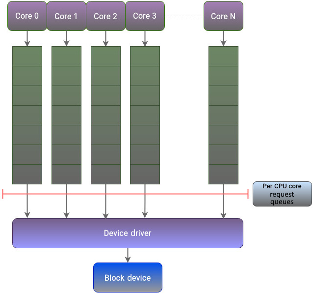
Figure 5.2 – The multi-queue framework

By using this approach, a CPU core can focus on executing its threads without worrying about the threads running on other cores. This approach resolves the limitations caused by the shared global lock and also minimizes the usage of interrupts and the need for cache coherency.

The blk-mq framework implements the following two-level queue design for handling I/O requests:

• Software staging queues: The software staging queues that are represented consist of one or more bio structures. A block device will have multiple software I/O submission queues, usually one per CPU core, and each queue will have a lock. A system with M sockets and N cores can have a minimum of M and a maximum of N queues. Each core submits I/O requests in its queue and doesn’t interact with other cores. These queues eventually fan into a single queue for the device driver. The I/O schedulers can operate on the requests in the staging queue to reorder or merge them. However, this reordering doesn’t matter as SSDs and NVMe drives don’t care if an I/O request is random or sequential. This scheduling happens only between requests in the same queue, so no locking mechanism is required.
• Hardware dispatch queues: The number of hardware queues that can be supported depends on the number of hardware contexts that are supported by the hardware and its corresponding device driver. However, it should be noted that the maximum number of hardware queues will not exceed the number of cores in the system. The number of software staging queues can be less than, greater than, or equal to the number of hardware queues. The hardware dispatch queues represent the last stage of the block layer’s code and act as a mediator before the requests get handed over to the device driver for their final execution. When an I/O request arrives at the block layer and there isn’t an I/O scheduler associated with the block device, blk-mq will send the request directly to the hardware queue.

The multi-queue API makes use of tags to indicate which request has been completed. Every request is identified by a tag, which is an integer value ranging from zero to the size of the dispatch queue. The block layer generates a tag, which is subsequently utilized by the device driver, eliminating the need for a duplicate identifier. Once the driver has finished processing the request, the tag is returned to the block layer to signal the completion of the operation. The following section highlights some of the major data structures that play a vital role in the implementation of the multi-queue block layer.

Looking at data structures

Here are some of the primary data structures that are essential to implement the multi-queue block layer:

• The first relevant data structure that’s used by the multi-queue framework is the blk_mq_register_dev structure, which contains all the necessary information required when registering a new block device to the block layer. It contains various fields that provide details about the driver’s capabilities and requirements.
• The blk_mq_ops data structure serves as a reference for the multi-queue block layer to access the device driver’s specific routines. This structure serves as an interface for communication between the driver and the blk-mq layer, enabling the driver to integrate seamlessly into the multi-queue processing framework.
• The software staging queues are represented by the blk_mq_ctx structure. This structure is allocated on a per-CPU core basis.
• The corresponding structure for hardware dispatch queues is defined by the blk_mq_hw_ctx struct. This represents the hardware context with which a request queue is associated.
• The task of mapping software staging queues to hardware dispatch queues is performed by the blk_mq_queue_map structure.
• The requests are created and sent to the block device through the blk_mq_submit_bio function.

The following figure paints a picture of how these functions are interconnected:

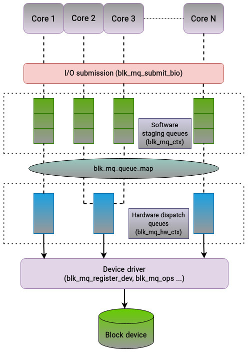
Figure 5.3 – Interplay of major structures in the multi-queue framework

To summarize, the multi-queue interface solves the limitations faced by the block layer when working with modern storage devices that have multiple queues. Historically, regardless of the capabilities of the underlying physical storage medium, the block layer maintained a single-request queue to handle I/O requests. On systems with multiple cores, this quickly turned into a major bottleneck. As the request queue was being shared between all CPU cores through a global lock, a considerable amount of time was spent by each CPU core waiting for the lock to be released by another core. To overcome this challenge, a new framework was developed to cater to the requirements of modern processors and storage devices. The multi-queue framework resolves the limitations of the block layer by segregating request queues for each CPU core. This framework leverages a dual queue design that is comprised of software staging queues and hardware dispatch queues.

With that, we have analyzed the multi-queue framework in the block layer. We will now shift our focus and explore the device mapper framework.

Looking at the device mapper framework

By default, managing physical block devices is rigid in that there are only a handful of ways in which an application can make use of them. When dealing with block devices, informed decisions have to be made regarding disk partitioning and space management to ensure optimal usage of available resources. In the past, features such as thin provisioning, snapshots, volume management, and encryption were exclusive to enterprise storage arrays. However, over time, these features have become crucial components of any local storage infrastructure. When operating with physical drives, it is expected that the upper layers of the operating system will possess the necessary capabilities to implement and sustain these functionalities. The Linux kernel provides the device mapper framework for implementing these concepts. The device mapper is used by the kernel to map physical block devices to higher-level virtual block devices. The primary goal of the device mapper framework is to create a high-level layer of abstraction on top of physical devices. The device mapper provides a mechanism to modify bio structures in transit and map them to block devices. The use of the device mapper framework lays the foundation for implementing features such as logical volume management.

The device mapper provides a generic way to create virtual layers of block devices on top of physical devices and implement features such as striping, mirroring, snapshots, and multipathing. Like most things in Linux, the functionality of the device mapper framework is divided into kernel space and user space. The policy-related work, such as defining physical-to-logical mappings, is contained in the user space, while the functions that implement the policies to establish these mappings lie in the kernel space.

The device mapper’s application interface is the ioctl system call. This system call adjusts the special file’s underlying device parameters. The logical devices that employ the device mapper framework are managed via the dmsetup command and the libdevmapper library, which implement the respective user interface, as depicted in the following figure:

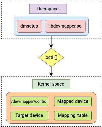
Figure 5.4 – Major components of the device mapper framework

If we run strace on the dmsetup command, we will see that it makes use of the libdevmapper library and the ioctl interface:

root@linuxbox:~# strace dmsetup ls
execve("/sbin/dmsetup", ["dmsetup", "ls"], 0x7fffbd282c58 /* 22 vars */) = 0
[..................]
access("/etc/ld.so.nohwcap", F_OK)      = -1 ENOENT (No such file or directory)
openat(AT_FDCWD, "/lib/x86_64-linux-gnu/libdevmapper.so.1.02.1", O_RDONLY|O_CLOEXEC) = 3
[...............…]
stat("/dev/mapper/control", {st_mode=S_IFCHR|0600, st_rdev=makedev(10, 236), ...}) = 0
openat(AT_FDCWD, "/dev/mapper/control", O_RDWR) = 3
openat(AT_FDCWD, "/proc/devices", O_RDONLY) = 4
[...............…]
ioctl(3, DM_VERSION, {version=4.0.0, data_size=16384, flags=DM_EXISTS_FLAG} => {version=4.41.0, data_size=16384, flags=DM_EXISTS_FLAG}) = 0
ioctl(3, DM_LIST_DEVICES, {version=4.0.0, data_size=16384, data_start=312, flags=DM_EXISTS_FLAG} => {version=4.41.0, data_size=528, data_start=312, flags=DM_EXISTS_FLAG, ...}) = 0
[..................]

Applications that establish mapped devices, such as LVM, communicate with the device mapper framework via the libdevmapper library. The libdevmapper library utilizes ioctl commands to transmit data to the /dev/mapper/control device. The /dev/mapper/control device is a specialized device that functions as a control mechanism for the device mapper framework.

From Figure 5.4, we can see that the device mapper framework in kernel space implements a modular architecture for storage management. The device mapper framework’s functionality consists of the following three major components:

• Mapped device
• Mapping table
• Target device

Let’s briefly look at their respective roles.

Looking at the mapped device

A block device, such as a whole disk or an individual partition, can be mapped to another device. The mapped device is a logical device provided by the device mapper driver and usually exists in the /dev/mapper directory. Logical volumes in LVM are examples of mapped devices. The mapped device is defined in drivers/md/dm-core.h. If we look at this definition, we will come across a familiar structure:

struct mapped_device {
[……..]
struct gendisk *disk;
[………..]

The gendisk structure, as explained in Chapter 4, represents the notion of a physical hard disk in the kernel.

Looking at the mapping table

A mapped device is defined by a mapping table. This mapping table represents a mapping from a mapped device to target devices. A mapped device is defined by a table that describes how each range of logical sectors of the device should be mapped, using a device table mapping that is supported by the device mapper framework. The mapping table defined in drivers/md/dm-core.h contains a pointer to the mapped device:

struct dm_table {
        struct mapped_device *md;
[……………..]

This structure allows mappings to be created, modified, and deleted in the device mapper stack. Details about the mapping table can be viewed by running the dmsetup command.

Looking at the target device

As explained earlier, the device mapper framework creates virtual block devices by defining mappings on physical block devices. Logical devices are created using “targets,” which can be thought of as modularized plugins. Different mapping types, such as linear, mirror, snapshot, and others, can be created using these targets. Data is passed from the virtual block device to the physical block device through these mappings. The target device structure is defined in include/linux/device-mapper.h. The unit that’s used for mapping is a sector:

struct dm_target {
        struct dm_table *table;
        sector_t begin;
        sector_t len;
[………….]

The device mapper can be a bit confusing to understand, so let’s illustrate a simple use case of the building blocks that we explained previously. We’re going to use the linear target, which lays the foundation of logical volume management. As discussed earlier, we’re going to use the dmsetup command for this purpose as it implements the user-space functionality of the device mapper. We’re going to create a linear mapping target called dm_disk. If you plan on running the following commands, make sure that you run them on a blank disk. Here, I’ve used two disks, sdc and sdd (you can use any disk for the exercise, so long it’s empty!). Note that once you press Enter after the dmsetup create commands, it will prompt you for input. The sdc and sdd disks are referred to using their respective major and minor numbers. You can find out the major and minor numbers for your disk using lsblk. The major and minor numbers for sdc are 8 and 32, expressed as 8:32. Similarly, for sdd, this combination is expressed as 8:48. The rest of the input fields will be explained shortly. Once you’ve entered the required data, use Ctrl + D to exit. The following example will create a linear target of 5 GiB:

[root@linuxbox ~]# dmsetup create dm_disk
dm_disk: 0 2048000 linear 8:32 0
dm_disk: 2048000 8192000 linear 8:48 1024
[root@linuxbox ~]#
[root@linuxbox ~]# fdisk -l /dev/mapper/dm_disk
Disk /dev/mapper/dm_disk: 4.9 GiB, 5242880000 bytes, 10240000 sectors
Units: sectors of 1 * 512 = 512 bytes
Sector size (logical/physical): 512 bytes / 512 bytes
I/O size (minimum/optimal): 512 bytes / 512 bytes
[root@linuxbox ~]#

Here’s what we’ve done:

1. We have created a logical device called dm_disk by using specific portions or ranges from two physical disks, sdc and sdd.
2. The first line of input that we’ve entered, dm_disk: 0 2048000 linear 8:32 0, means that the first 2048000 sectors (0-2047999) of dm_disk will use the sectors of /dev/sdc, starting from sector 0. Therefore, the first 2048000 (0-2047999) sectors of sdc will be used by dm_disk.
3. The second line, dm_disk: 2048000 8192000 linear 8:48 1024, means that the next 8192000 sectors (after sector number 2047999) of dm_disk are being allocated from sdd. These 8192000 sectors from sdd will be allocated from sector number 1024 onward. If the disks do not contain any data, we can use any sector number here. If existing data is present, then the sectors should be allocated from an unused range.
4. The total number of sectors in dm_disk will be 8192000 + 2048000 = 10240000.
5. With a sector size of 512 bytes, the size of dm_disk will be (8192000 x 512) + (2048000 x 512) ≈ 5 GiB.

The 0-2047999 sector numbers of dm_disk are mapped from sdc, whereas the 2048000-10239999 sector numbers are mapped from sdd. The example we’ve discussed is a simple one, but it should be evident that we can map a logical device to any number of drives and implement different concepts.

The following figure summarizes what we explained earlier:

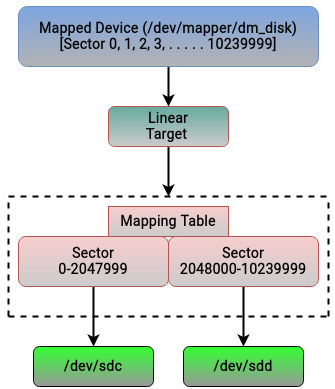
Figure 5.5 – Linear target mapping in the device mapper framework

The device mapper framework supports a wide variety of targets. Some of them are explained here:

• Linear: As we saw earlier, a linear mapping target can map a continuous range of blocks to another block device. This is the basic building block of logical volume management.
• Raid: The raid target is used to implement the concept of software raid. It is capable of supporting different raid types.
• Crypt: The crypt target is used to encrypt data on block devices.
• Stripe: The stripe target is used to create a striped device called (raid 0) across multiple underlying disks.
• Multipath: The multipath mapping target is utilized in storage environments where a host has multiple paths to a storage device. It allows a multipath device to be mapped.
• Thin: The thin target is used for thin provisioning – that is, creating devices larger than the size of the underlying physical device. The physical space is allocated only when written to.

As repeatedly mentioned earlier, the linear mapping target is most commonly implemented in LVM. Most Linux distributions use LVM by default for space allocation and partitioning. To the common user, LVM is probably one of the more well-known features of Linux. It should not be too difficult to see how the previously mentioned example can be applied to LVM or any other target for that matter.

As most of you should be aware, LVM is divided into three basic entities:

• Physical volume: The physical volume is at the lowest layer. The underlying physical disk or partition is a physical volume.
• Volume group: The volume group divides the space available in a physical volume into a sequence of chunks, called physical extents. A physical extent represents a contiguous range of blocks. It is the smallest unit of disk space that can be individually managed by LVM. By default, an extent size of 4 MB is used.
• Logical volume: From the space available in a volume group, logical volumes can be created. Logical volumes are typically divided into smaller chunks of data, each known as a logical extent. Since LVM utilizes linear target mapping, there is a direct correspondence between physical and logical extents. Consequently, a logical volume can be viewed as a mapping that’s established by LVM that associates logical extents with physical ones. This can be visualized in the following figure:

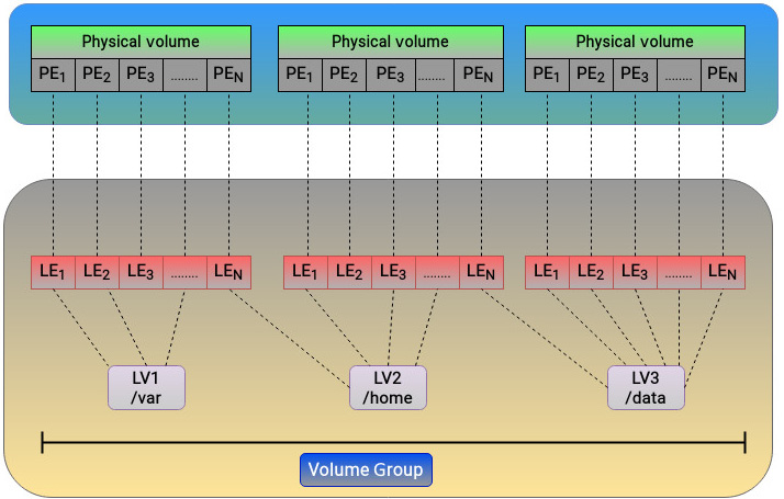
Figure 5.6 – LVM architecture

The logical volumes, as we all know, can be treated like any regular block device, and filesystems can be created on top of them. A single logical volume that spans multiple physical disks is similar to RAID-0. The type of mapping to be used between physical and logical extents is determined by the target. As LVM is based on a linear target, there is a one-to-one mapping relationship between physical and logical extents. Let’s say we were to use the dm-raid target and configure RAID-1 to do mirroring between multiple block devices. In that case, multiple physical extents will map to a single logical extent.

Let’s wrap up our discussion of the device mapper framework by mapping some key facts in our minds. The device mapper framework plays a vital role in the kernel and is responsible for implementing several key concepts in the storage hierarchy. The kernel uses the device mapper framework to map physical block devices to higher-level virtual block devices. The functionality of the device mapper framework is split into user space and kernel space. The user-space interface consists of the libdevmapper library and the dmsetup utility. The kernel part consists of three major components: the mapped device, mapping table, and target device. The device mapper framework provides the basis for several important technologies in Linux, such as LVM. LVM provides a thin layer of abstraction above physical disks and partitions. This abstraction layer allows storage administrators to easily resize filesystems based on their space requirements, providing them with a high level of flexibility. Before concluding this chapter, let’s briefly touch on the caching mechanisms that are employed by the block layer.

Looking at multi-tier caching mechanisms in the block layer

The performance of physical storage is usually orders of magnitude slower than that of processors and memory. The Linux kernel is well aware of this limitation. Hence, it uses the available memory as a cache and performs all operations in memory before writing all data to the underlying disks. This caching mechanism is the default behavior of the kernel and it plays a central role in improving the performance of block devices. This also positively contributes toward improving the system’s overall performance.

Although solid state and NVMe drives are now commonplace in most storage infrastructures, the traditional spinning drives are still being used for cases where capacity is required and performance is not a major concern. When we talk about drive performance, random workloads are the Achilles heel of spinning mechanical drives. In comparison, the performance of flash drives does not suffer from such limitations, but they are far more expensive than mechanical drives. Ideally, it would be nice to get the advantages of both media types. Most storage environments are hybrid and try to make efficient use of both types of drives. One of the most common techniques is to place hot or frequently used data on the fastest physical medium and move cold data to slower mechanical drives. Most enterprise storage arrays offer built-in storage tiering features that implement this caching functionality.

The Linux kernel is also capable of implementing such a cache solution. The kernel offers several options to combine the capacity offered by spinning mechanical drives with the speed of access offered by SSDs. As we saw earlier, the device mapper framework offers a wide variety of targets that add functionalities on top of block devices. One such target is the dm-cache target. The dm-cache target can be used to improve the performance of mechanical drives by migrating some of its data to faster drives, such as SSDs. This approach is a bit contrary to the kernel’s default caching mechanism, but it can be of significant use in some cases.

Most cache mechanisms offer the following operational modes:

• Write-back: This mode caches newly written data but does not write it immediately to the target device.
• Write-through: In this mode, new data is written to the target while still retaining it in the cache for subsequent reads.
• Write-around: This mode implements read-only caching. Data written to the device goes directly to the slower mechanical drive and is not written to the fast SSD.
• Pass-through: To enable pass-through mode, the cache needs to be clean. Reading is served from the origin device that bypasses the cache. Writing is forwarded to the origin device and invalidates the cache block.

The dm-cache target supports all the previously mentioned modes, except write-around. The required functionality is implemented through the following three devices:

• Origin device: This will always be the slow primary storage device
• Cache device: This is a high-performing drive, usually an SSD
• Metadata device: Although this is optional and this information can also be saved on the fast cache device, this device is used for keeping track of all the metadata information, such as which disk blocks are in the cache, which blocks are dirty, and so on

Another similar caching solution is dm-writecache, which is also a device mapper target. As its name suggests, the main focus of dm-writecache is strictly write-back caching. It only caches write operations and does not perform any read or write-through caching. The thought process for not caching reads is that read data should already be in the page cache. The write operations are cached on the faster storage device and then migrated to the slower disk in the background.

Another notable solution that has gained widespread popularity is bcache. The bcache solution supports all four caching modes defined previously. bcache uses a far more complex approach and lets all sequential operations go to the mechanical drives by default. Since SSDs excel at random operations, there generally won’t be many benefits to caching large sequential operations on SSDs. Hence, bcache detects sequential operations and skips them. The writers for bcache compare it to the L2 adaptive replacement cache (ARC) in ZFS. The bcache project has also led to the development of the Bcachefs filesystem.