In the final section of this chapter, we will learn about computing correlations using pandas and SciPy. We will look at how to use pandas and SciPy to compute correlations in datasets, and also explore some statistical tests to detect correlation.
In this section, I have used Pearson's correlation coefficient, which quantifies how strongly two variables are linearly correlated. This is a unitless number that takes values between -1 and 1. The sign of the correlation coefficient indicates the direction of the relationship. A positive r indicates that as one variable increases, the other tends to increase; while a negative r indicates that as one variable increases, the other tends to decrease. The magnitude indicates the strength of the relationship. If r is close to 1 or -1, then the relationship is almost a perfect linear relationship, while an r that is close to 0 indicates no linear relationship. The NumPy corrcoef() function computes the number for two NumPy arrays.
So, here's the correlation coefficient's definition. We're going to work with what's known as the Boston housing price dataset. This is known as a toy dataset, and is often used for evaluating statistical learning methods. I'm only interested in looking at correlations between the variables in this dataset.
We will use the following steps:
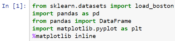
- We will first load up all the required libraries, as follows:
- We will then load in the dataset using the following code:

- Then, we will print the dataset information, so that we can have a look at it, as follows:
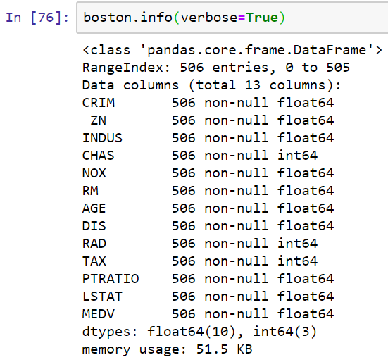
So, these attributes tell us what this dataset contains. It has a few different variables such as, for example, the crime rate by town, the proportion of residential land zones, non-retail business acres, and others. Therefore, we have a number of different attributes for you to play with.
- We will now load the actual dataset, as follows:
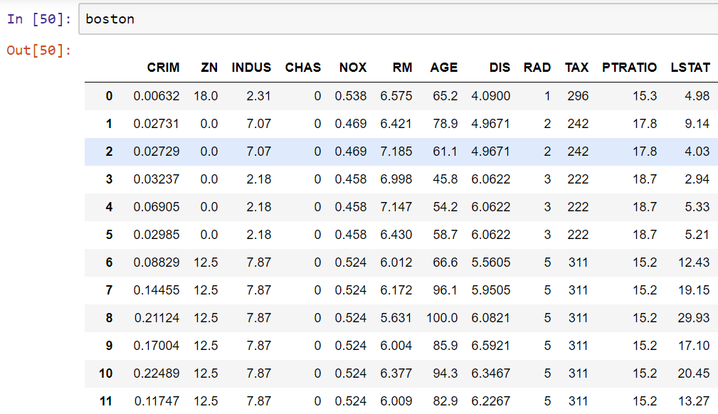
This is going to very useful to us. Now, let's take a look at the correlation between the two variables.
- We're going to import the corrcoef() function, and we're going to look at one of the columns from this dataset as if it were a NumPy array, as follows:
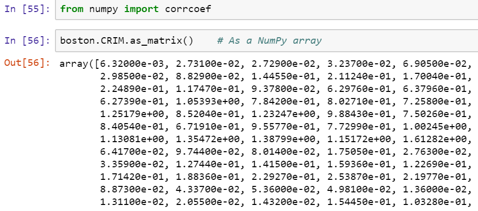
It started out as a NumPy array, but it's perfectly fine to just grab a pandas series and turn it into an array.
- Now we're going to take corrcoef(), and compute the correlation between the crime rate and the price:
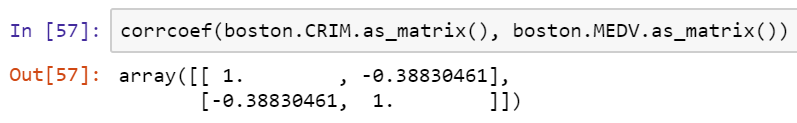
We can see that the numbers in the matrix are the same.
The number in the off-diagonal entries corresponds to the correlation between the two variables. Therefore, there is a negative relationship between crime rate and price, which is not surprising. As the crime rate increases, you would expect the price to decrease. But this is not a very strong correlation. We often want correlations not just for two variables, but for many combinations of two variables. We can use the pandas DataFrame corr() method to compute what's known as the correlation matrix. This matrix contains correlations for every combination of variables in our dataset.
- So, let's go ahead and compute a correlation matrix for the Boston dataset, using the corr() function:
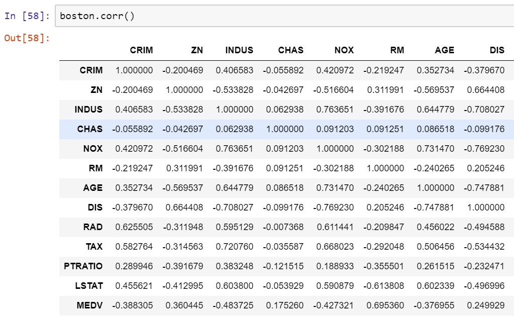
These are all correlations. Every entry off the diagonal will have a corresponding entry on the other side of the diagonal—this is a symmetric matrix. Now, while this matrix contains all the data that we might want, it is very difficult to read.
- So, let's use a package called seaborn, as this is going to allow us to plot a heatmap. A heatmap has colors with differing intensities for how large or small a number tends to be. So, we compute a heatmap and plot it as follows:
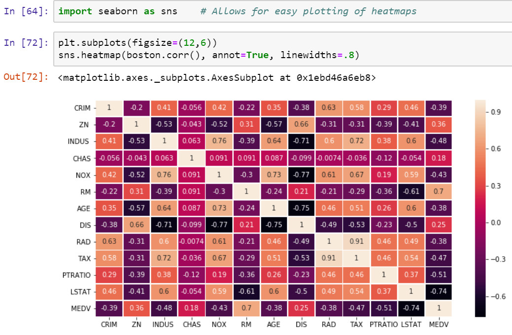
The preceding screenshot shows the resulting map. Here, black indicates correlations close to -1, and very light colors indicate correlations that are close to 1. From this heatmap, we can start to see some patterns.