Search icon CANCEL
Subscription
0
Cart icon
Cart
Close icon
You have no products in your basket yet
Save more on your purchases!
Savings automatically calculated. No voucher code required
Arrow left icon
All Products
Best Sellers
New Releases
Books
Videos
Audiobooks
Learning Hub
Newsletters
Free Learning
Arrow right icon
Arrow up icon
GO TO TOP
Training Systems using Python Statistical Modeling

You're reading from  Training Systems using Python Statistical Modeling

Product type Book
Published in May 2019
Publisher Packt
ISBN-13 9781838823733
Pages 290 pages
Edition 1st Edition
Languages
Author (1):
Curtis Miller Curtis Miller
Profile icon Curtis Miller
Toc

Bayesian analysis for means

Now we'll move on to discussing Bayesian methods for analyzing the means of quantitative data. This section is similar to the previous one on Bayesian methods for analyzing proportions, but it focuses on the means of quantitative data. Here, we look at constructing credible intervals and performing hypothesis testing.

Suppose that we assume that our data was drawn from a normal distribution with an unknown mean, μ, and an unknown variance, σ2. The conjugate prior, in this case, will be the normal inverse gamma (NIG) distribution. This is a two-dimensional distribution, and gives a posterior distribution for both the unknown mean and the unknown variance.

In this section, we only care about what the unknown mean is. We can get a marginal distribution for the mean from the posterior distribution, which depends only on the mean. The variance no longer appears in the marginal distribution. We can use this distribution for our analysis.

So, we say that the mean and the standard deviation, both of these things being unknown, were drawn from a NIG distribution with the parameters of μ0, μ, α, and β. This can be represented using the following formula:

The posterior distribution after you have collected data can be represented as follows:

In this case, I'm interested in the marginal distribution of the mean, μ, under the posterior distribution. The prior marginal distribution of μ is t(2α), which means that it follows a t-distribution with two alpha degrees of freedom; this is the posterior marginal distribution of the following formula:

Here, it is t(2α + n).

This is all very complicated, so I've written five helper functions, which are as follows:

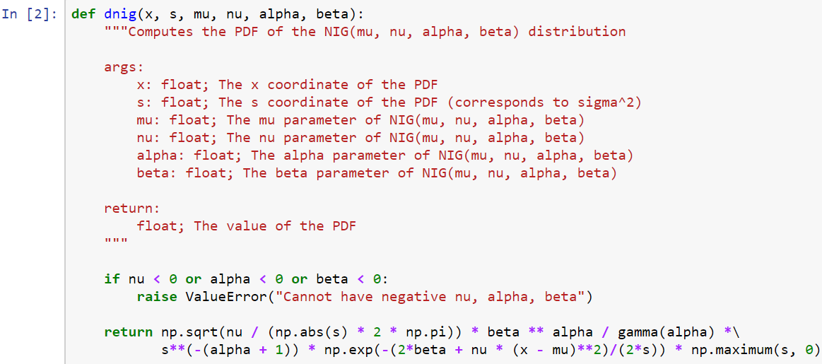
  • Compute the probability density function (PDF) of (μ,σ2), which is useful for plotting.
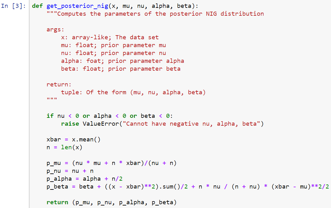
  • Compute the parameters of the posterior distribution of (μ,σ2).
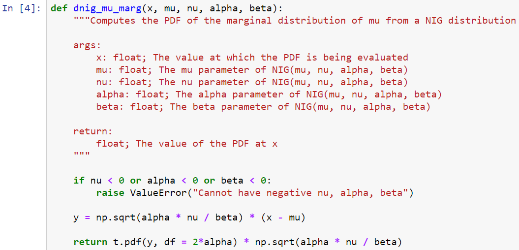
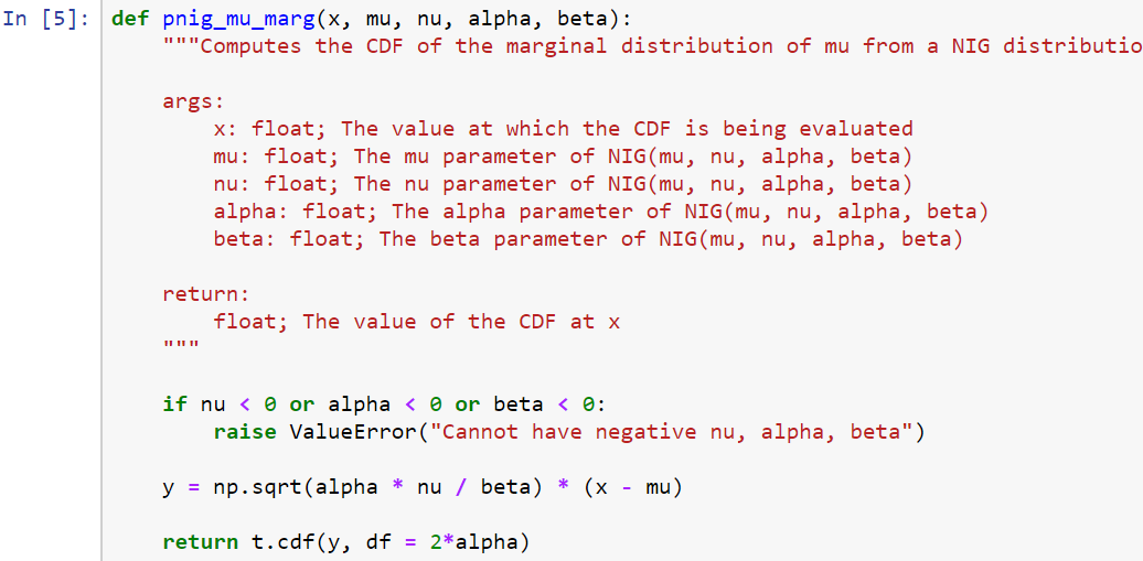
  • Compute the PDF and CDF of the marginal distribution of μ (for either the prior or posterior distribution).
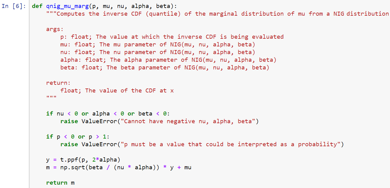
  • Compute the inverse CDF of the marginal distribution of μ (for either the prior or posterior distribution).
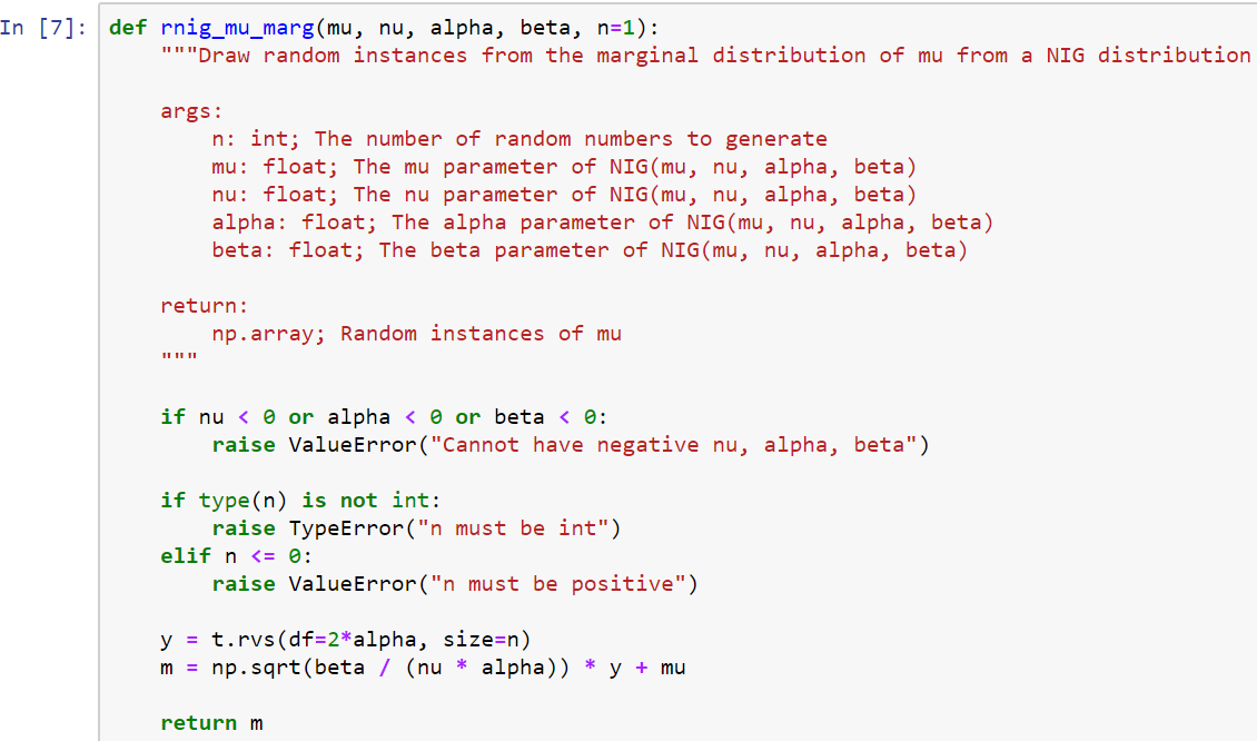
  • Simulate a draw from the marginal distribution of μ (for either the prior or posterior distribution).

We will apply these functions using the following steps:

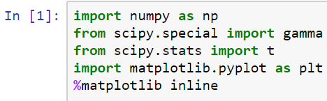
  1. So, first, we're going to need these libraries:
  1. Then, the dnig() function computes the density of the normal inverse gamma distributionthis is helpful for plotting, as follows:
  1. The get_posterior_nig() function will get the parameters of the posterior distribution, where x is our data; and these four parameters specify the parameters of the prior distribution, but will be returned as a tuple that contains the parameters of the posterior distribution:
  1. The dnig_mu_marg() function is the density function of the marginal distribution for μ. It will be given a floating-point number that you want to evaluate the PDF on. This will be useful if you want to plot the marginal distribution of μ:
  1. The pnig_mu_marg() function computes the CDF of the marginal distribution; that is, the probability of getting a value less than or equal to your value of x, which you pass to the function. This'll be useful if you want to do things such as hypothesis testing or computing the probability that a hypothesis is true under the posterior distribution:
  1. The qunig_mu_marg() function will be the inverse CDF, however, you give it a probability, and it will give you the quantile associated with that probability. This is a function that's going to be useful if you want to construct, say, credible intervals:
  1. Finally, the rnig_mu_marg() function draws random numbers from the marginal distribution of μ from a normal inverse gamma distribution, so this'll be useful if you want to sample from the posterior distribution of μ:
  1. Now, we will perform a short demonstration of what the dnig() function does, so you can get an idea of what the normal inverse gamma distribution looks like, using the following code:

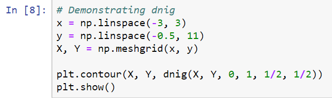
This results in the following output:

This plot gives you a sense of what the normal inverse gamma looks like. Therefore, most of the density is concentrated in this region, but it starts to spread out.

Credible intervals for means

Getting a credible interval for the mean is the same as the one for proportions, except that we will work with the marginal distribution for just the unknown mean from the posterior distribution.

Let's repeat a context that we used in the Computing confidence intervals for means section of this chapter. You are employed by a company that's fabricating chips and other electronic components. The company wants you to investigate the resistors it's using to produce its components. These resistors are being manufactured by an outside company and they've been specified as having a particular resistance. They want you to ensure that the resistors being produced and sent to them are high quality productsspecifically, that when they are labeled with a resistance level of 1,000 Ω, then they do in fact have a resistance of 1,000 Ω. So, let's get started, using the following steps:

  1. We will use the same dataset as we did in the Computing confidence intervals for means section.
  1. Now, we're going to use the NIG (1, 1, 1/2, 0.0005) distribution for our prior distribution. You can compute the parameters of the posterior distribution using the following code:

When the parameters of the distribution are computed, it results in the following output:

It looks as if the mean has been moved; you now have 105 observations being used as your evidence.

  1. Now, let's visualize the prior and posterior distributionspecifically, their marginal distributions:

Blue represents the prior distribution, and red represents the posterior distribution. It appears that the prior distribution was largely uninformative about where the true resistance was, while the posterior distribution strongly says that the resistance is approximately 0.99.

  1. Now, let's use this to compute a 95% credible interval for the mean of μ. I have written a function that will do this for you, where you feed it data and also the parameters of the prior distribution, and it will give you a credible interval with a specified level of credibility. Let's run this function as follows:
  1. Now, let's compute the credible interval:

Here, what we notice is that 1 is not in this credible interval, so there's a 95% chance that the true resistance level is between 0.9877 and 0.9919.

Bayesian hypothesis testing for means

Hypothesis testing is similar, in principle, to what we have done previously; only now, we are using the marginal distribution of the mean from the posterior distribution. We compute the probability that the mean lies in the region corresponding to the hypothesis being true.

So, now, you want to test whether the true mean is less than 1,000 Ω. To do this, we get the parameters of the posterior distribution, and then feed these to the pnig_mu_marg() function:

We end up with a probability that is almost 1. It is all but certain that the resistors are not properly calibrated.

Testing with two samples

Suppose that we want to compare the means of two populations. We start by assuming that the parameters of the two populations are independent and compute their posterior distributions, including the marginal distributions of the means. Then, we use Monte Carlo methods, similar to those used previously, to estimate the probability that one mean is less than the other. So, let's now take a look at two-sample testing.

Your company has decided that it no longer wants to stick with this manufacturer. They want to start producing resistors in-house, and they're looking at different methods for producing these resistors. Right now, they have two manufacturing processes known as process A and process B, and you want to know whether the mean for process A is less than the mean for process B. So, what we'll do is use Monte Carlo methods, as follows:

  1. Collect data from both processes and compute the posterior distributions for both μA and μB.
  2. Simulate random draws of μA and μB from the posterior distributions.
  3. Compute how often μA is less than μB to estimate the probability that μA > μB.

So, first, let's get the dataset for the two processes:

We get the posterior distributions for both processes as follows:

Now, let's simulate 1,000 draws from the posterior distributions:

Here are the random μA values:

Here are the random μB values:

Here is when μA is less than μB:

Finally, we add these up and take the mean, as follows:

We can see that about 65.8% of the time μA is less than μB. This is higher than 50%, which suggests that μA is probably less than μB, but this is not a very actionable probability. 65.8% is not a probability high enough to strongly suggest a change needs to be made.

So, that's it for Bayesian statistics for now. We will now move on to computing correlations in datasets.

You have been reading a chapter from
Training Systems using Python Statistical Modeling
Published in: May 2019 Publisher: Packt ISBN-13: 9781838823733
Register for a free Packt account to unlock a world of extra content!
A free Packt account unlocks extra newsletters, articles, discounted offers, and much more. Start advancing your knowledge today.
Unlock this book and the full library FREE for 7 days
Get unlimited access to 7000+ expert-authored eBooks and videos courses covering every tech area you can think of
Renews at $15.99/month. Cancel anytime