Chapter 6: Unsupervised Learning
Activity 20: Perform DIANA, AGNES, and k-means on the Built-In Motor Car Dataset
Solution:
- Attach the cluster and factoextra packages:
library(cluster)
library(factoextra)
- Load the dataset:
df <- read.csv("mtcars.csv")
- Set the row names to the values of the X column (the state names). Remove the X column afterward:
rownames(df) <- df$X
df$X <- NULL
Note
The row names (states) become a column, X, when you save it as a CSV file. So, we need to change it back, as the row names are used in the plot in step 7.
- Remove those rows with missing data and standardize the dataset:
df <- na.omit(df)
df <- scale(df)
- Implement divisive hierarchical clustering using DIANA. For easy comparison, document the dendrogram output. Feel free to experiment with different distance metrics:
dv <- diana(df,metric = "manhattan", stand = TRUE)
plot(dv)
The output is as follows:

Figure 6.41: Banner from diana()
The next plot is as follows:

Figure 6.42: Dendrogram from diana()
- Implement bottom-up hierarchical clustering using AGNES. Take note of the dendrogram created for comparison purposes later on:
agn <- agnes(df)
pltree(agn)
The output is as follows:

Figure 6.43: Dendrogram from agnes()
- Implement k-means clustering. Use the elbow method to determine the optimal number of clusters:
fviz_nbclust(mtcars, kmeans, method = "wss") +
geom_vline(xintercept = 4, linetype = 2) +
labs(subtitle = "Elbow method")
The output is as follows:

Figure 6.44: Optimal clusters using the elbow method
- Perform k-means clustering with four clusters:
k4 <- kmeans(df, centers = 4, nstart = 20)
fviz_cluster(k4, data = df)
The output is as follows:

Figure 6.45: k-means with four clusters
- Compare the clusters, starting with the smallest one. The following are your expected results for DIANA, AGNES, and k-means, respectively:
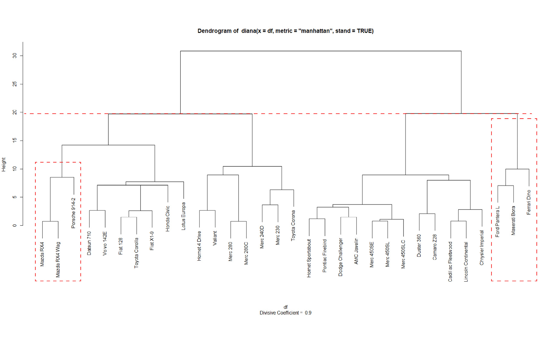
Figure 6.46: Dendrogram from running DIANA, cut at 20
If we consider cutting the DIANA tree at height 20, the Ferrari is clustered together with the Ford and the Maserati (the smallest cluster):
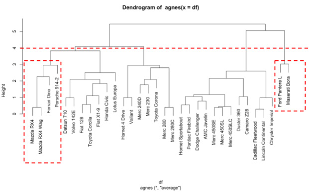
Figure 6.47: Dendrogram from agnes, cut at 4
Meanwhile, cutting the AGNES dendrogram at height 4 results in the Ferrari being clustered with the Mazda RX4, the Mazda RX4 Wag, and the Porsche. k-means clusters the Ferrari with the Mazdas, the Ford, and the Maserati.
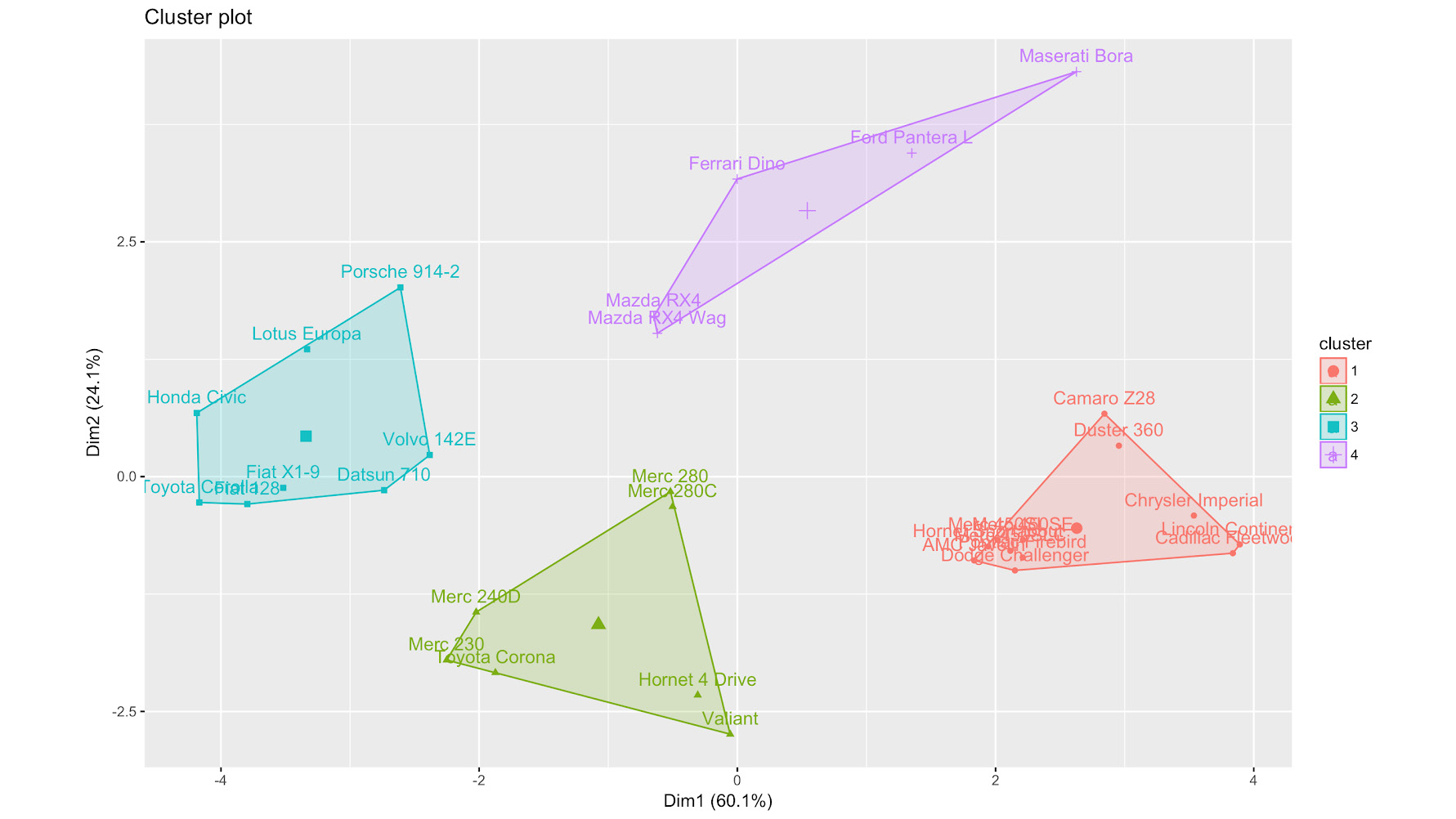
Figure 6.48: kmeans clustering
Clearly, the choice of clustering technique and algorithms results in different clusters being created. It is important to apply some domain knowledge to determine the most valuable end results.


