High-level ML system design

When you get down to the nuts and bolts of building your solution, there are so many options for tools, tech, and approaches that it can be very easy to be overwhelmed. However, as alluded to in the previous sections, a lot of this complexity can be abstracted to understand the bigger picture via some back-of-the-envelope architecture and designs. This is always a useful exercise once you know what problem you will try and solve, and it is something I recommend doing before you make any detailed choices about implementation.

To give you an idea of how this works in practice, what follows are a few worked-through examples where a team has to create a high-level ML systems design for some typical business problems. These problems are similar to ones I have encountered before and will likely be similar to ones you will encounter in your own work.

Example 1: Batch anomaly detection service

You work for a tech-savvy taxi ride company with a fleet of thousands of cars. The organization wants to start making ride times more consistent and understand longer journeys in order to improve the customer experience and, thereby, increase retention and return business. Your ML team is employed to create an anomaly detection service to find rides that have unusual ride time or ride length behaviors. You all get to work, and your data scientists find that if you perform clustering on sets of rides using the features of ride distance and time, you can clearly identify outliers worth investigating by the operations team. The data scientists present the findings to the CTO and other stakeholders before getting the go-ahead to develop this into a service that will provide an outlier flag as a new field in one of the main tables of the company’s internal analysis tool.

In this example, we will simulate some data to show how the taxi company’s data scientists could proceed. In the repository for the book, which can be found at https://github.com/PacktPublishing/Machine-Learning-Engineering-with-Python-Second-Edition, if you navigate to the folder Chapter01, you will see a script called clustering_example.py. If you have activated the conda environment provided via the mlewp-chapter01.yml environment file, then you can run this script with:

python3 clustering_example.py

After a successful run you should see that three files are created: taxi-rides.csv, taxi-labels.json, and taxi-rides.png. The image in taxi-rides.png should look something like that shown in Figure 1.4.

We will walk through how this script is built up:

1. First, let’s define a function that will simulate some ride distances based on the random distribution given in numpy and return a numpy array containing the results. The reason for the repeated lines is so that we can create some base behavior and anomalies in the data, and you can clearly compare against the speeds we will generate for each set of taxis in the next step:

   import numpy as np
   from numpy.random import MT19937
   from numpy.random import RandomState, SeedSequence
   rs = RandomState(MT19937(SeedSequence(123456789)))
   
   # Define simulate ride data function
   def simulate_ride_distances():
       ride_dists = np.concatenate(
           (
               10 * np.random.random(size=370),
               30 * np.random.random(size=10), # long distances
               10 * np.random.random(size=10), # same distance
               10 * np.random.random(size=10) # same distance
           )
       )
       return ride_dists
   

2. We can now do the exact same thing for speeds, and again we have split the taxis into sets of 370, 10, 10, and 10 so that we can create some data with “typical” behavior and some sets of anomalies, while allowing for clear matching of the values with the distances function:

   def simulate_ride_speeds():
       ride_speeds = np.concatenate(
           (
               np.random.normal(loc=30, scale=5, size=370),
               np.random.normal(loc=30, scale=5, size=10),
               np.random.normal(loc=50, scale=10, size=10),
               np.random.normal(loc=15, scale=4, size=10) 
           )
       )
       return ride_speeds
   

3. We can now use both of these helper functions inside a function that will call them and bring them together to create a simulated dataset containing ride IDs, speeds, distances, and times. The result is returned as a pandas DataFrame for use in modeling:

   def simulate_ride_data():
       # Simulate some ride data …
       ride_dists = simulate_ride_distances()
       ride_speeds = simulate_ride_speeds()
       ride_times = ride_dists/ride_speeds
       # Assemble into Data Frame
       df = pd.DataFrame(
           {
             'ride_dist': ride_dists,
             'ride_time': ride_times,
             'ride_speed': ride_speeds
           }
       )
       ride_ids = datetime.datetime.now().strftime("%Y%m%d") +\
                  df.index.astype(str)
       df['ride_id'] = ride_ids
       return df
   

4. Now, we get to the core of what data scientists produce in their projects, which is a simple function that wraps some sklearn code to return a dictionary with the clustering run metadata and results.

   We include the relevant imports here for ease:

   from sklearn.preprocessing import StandardScaler
   from sklearn.cluster import DBSCAN
   from sklearn import metrics 
   
   def cluster_and_label(data, create_and_show_plot=True):
       data = StandardScaler().fit_transform(data)
       db = DBSCAN(eps=0.3, min_samples=10).fit(data)
       # Find labels from the clustering
       core_samples_mask = np.zeros_like(db.labels_,dtype=bool)
       core_samples_mask[db.core_sample_indices_] = True
       labels = db.labels_
       # Number of clusters in labels, ignoring noise if present.
       n_clusters_ = len(set(labels)) -
                            (1 if -1 in labels else 0)
       n_noise_ = list(labels).count(-1)
       run_metadata = {
           'nClusters': n_clusters_,
           'nNoise': n_noise_,
           'silhouetteCoefficient':
            metrics.silhouette_score(data, labels),
           'labels': labels,
       }
       if create_and_show_plot:
           plot_cluster_results(data, labels, core_samples_mask,
                                n_clusters_)
       else:
           pass
       return run_metadata
   

   Note that the function in step 4 leverages a utility function for plotting that is shown below:

   import matplotlib.pyplot as plt
   
   def plot_cluster_results(data, labels, core_samples_mask,
                            n_clusters_):
       fig = plt.figure(figsize=(10, 10))
       # Black removed and is used for noise instead.
       unique_labels = set(labels)
       colors = [plt.cm.cool(each) for each in np.linspace(0, 1,
                 len(unique_labels))]
       for k, col in zip(unique_labels, colors):
           if k == -1:
               # Black used for noise.
               col = [0, 0, 0, 1]
           class_member_mask = (labels == k)
           xy = data[class_member_mask & core_samples_mask]
           plt.plot(xy[:, 0], xy[:, 1], 'o',
                    markerfacecolor=tuple(col),
                    markeredgecolor='k', markersize=14)
           xy = data[class_member_mask & ~core_samples_mask]
           plt.plot(xy[:, 0], xy[:, 1], '^',
                    markerfacecolor=tuple(col),
                    markeredgecolor='k', markersize=14)
       plt.xlabel('Standard Scaled Ride Dist.')
       plt.ylabel('Standard Scaled Ride Time')
       plt.title('Estimated number of clusters: %d' % n_clusters_)
       plt.savefig('taxi-rides.png')
   

   Finally, this is all brought together at the entry point of the program, as shown below:

   import logging
   logging.basicConfig()
   logging.getLogger().setLevel(logging.INFO)
   
   if __name__ == "__main__":
       import os
       # If data present, read it in
       file_path = 'taxi-rides.csv'
       if os.path.exists(file_path):
           df = pd.read_csv(file_path)
       else:
           logging.info('Simulating ride data')
           df = simulate_ride_data()
           df.to_csv(file_path, index=False)
       X = df[['ride_dist', 'ride_time']]
       
       logging.info('Clustering and labelling')
       results = cluster_and_label(X, create_and_show_plot=True)
       df['label'] = results['labels']
       
       logging.info('Outputting to json ...')
       df.to_json('taxi-labels.json', orient='records')
   

This script, once run, creates a dataset showing each simulated taxi journey with its clustering label in taxi-labels.json, as well as the simulated dataset in taxi-rides.csv and the plot showing the results of the clustering in taxi-rides.png, as shown in Figure 1.4.

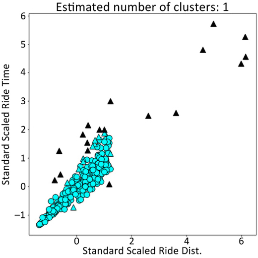
Figure 1.4: An example set of results from performing clustering on some taxi ride data.

Now that you have a basic model that works, you have to start thinking about how to pull this into an engineered solution – how could you do it?

Well, since the solution here will support longer-running investigations by another team, there is no need for a very low-latency solution. The stakeholders agree that the insights from clustering can be delivered at the end of each day. Working with the data science part of the team, the ML engineers (led by you) understand that if clustering is run daily, this provides enough data to give appropriate clusters, but doing the runs any more frequently could lead to poorer results due to smaller amounts of data. So, a daily batch process is agreed upon.

The next question is, how do you schedule that run? Well, you will need an orchestration layer, which is a tool or tools that will enable you to schedule and manage pre-defined jobs. A tool like Apache Airflow would do exactly this.

What do you do next? Well, you know the frequency of runs is daily, but the volume of data is still very high, so it makes sense to leverage a distributed computing paradigm. Two options immediately come to mind and are skillsets that exist within the team, Apache Spark and Ray. To provide as much decoupling as possible from the underlying infrastructure and minimize the refactoring of your code required, you decide to use Ray. You know that the end consumer of the data is a table in a SQL database, so you need to work with the database team to design an appropriate handover of the results. Due to security and reliability concerns, it is not a good idea to write to the production database directly. You, therefore, agree that another database in the cloud will be used as an intermediate staging area for the data, which the main database can query against on its daily builds.

It might not seem like we have done anything technical here, but actually, you have already performed the high-level system design for your project. The rest of this book tells you how to fill in the gaps in the following diagram!

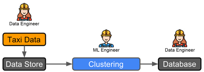
Figure 1.5: Example 1 workflow.

Let’s now move on to the next example!

Example 2: Forecasting API

In this example, you work for the logistics arm of a large retail chain. To maximize the flow of goods, the company would like to help regional logistics planners get ahead of particularly busy periods and avoid product sell-outs. After discussions with stakeholders and subject matter experts across the business, it is agreed that the ability for planners to dynamically request and explore forecasts for particular warehouse items through a web-hosted dashboard is optimal. This allows the planners to understand likely future demand profiles before they make orders.

The data scientists come good again and find that the data has very predictable behavior at the level of any individual store. They decide to use the Facebook Prophet library for their modeling to help speed up the process of training many different models. In the following example we will show how they could do this, but we will not spend time optimizing the model to create the best predictive performance, as this is just for illustration purposes.

This example will use the Kaggle API in order to retrieve an exemplar dataset for sales in a series of different retail stores. In the book repository under Chapter01/forecasting there is a script called forecasting_example.py. If you have your Python environment configured appropriately you can run this example with the following command at the command line:

python3 forecasting_example.py

The script downloads the dataset, transforms it, and uses it to train a Prophet forecasting model, before running a prediction on a test set and saving a plot. As mentioned, this is for illustration purposes only and so does not create a validation set or perform any more complex hyperparameter tuning than the defaults provided by the Prophet library.

To help you see how this example is pieced together, we will now break down the different components of the script. Any functionality that is purely for plotting or logging is excluded here for brevity:

1. If we look at the main block of the script, we can see that the first steps all concern reading in the dataset if it is already in the correct directory, or downloading and then reading it in otherwise:

   import pandas as pd
   
   if __name__ == "__main__":
       import os
       file_path = train.csv
       if os.path.exists(file_path):
           df = pd.read_csv(file_path)
       else:
           download_kaggle_dataset()
           df = pd.read_csv(file_path)
   

2. The function that performed the download used the Kaggle API and is given below; you can refer to the Kaggle API documentation to ensure this is set up correctly (which requires a Kaggle account):

   import kaggle
   
   def download_kaggle_dataset( kaggle_dataset: str ="pratyushakar/
                                rossmann-store-sales" ) -> None:
       api = kaggle.api
       kaggle.api.dataset_download_files(kaggle_dataset, path="./",
                                         unzip=True, quiet=False)
   

3. Next, the script calls a function to transform the dataset called prep_store_data. This is called with two default values, one for a store ID and the other specifying that we only want to see data for when the store was open. The definition of this function is given below:

   def prep_store_data(df: pd.DataFrame, 
                       store_id: int = 4, 
                       store_open: int = 1) -> pd.DataFrame:
       df['Date'] = pd.to_datetime(df['Date'])
       df.rename(columns= {'Date':'ds','Sales':'y'}, inplace=True)
       df_store = df[
           (df['Store'] == store_id) & 
           (df['Open'] == store_open)
           ].reset_index(drop=True)
       return df_store.sort_values('ds', ascending=True)
   

4. The Prophet forecasting model is then trained on the first 80% of the data and makes a prediction on the remaining 20% of the data. Seasonality parameters are provided to the model in order to guide its optimization:

   seasonality = {
       'yearly': True,
       'weekly': True,
       'daily': False
   }
   predicted, df_train, df_test, train_index = train_predict(
       df = df,
       train_fraction = 0.8,
       seasonality=seasonality
   )
   

   The definition of the train_predict method is given below, and you can see that it wraps some further data prep and the main calls to the Prophet package:

   def train_predict(df: pd.DataFrame, train_fraction: float, 
                     seasonality: dict) -> tuple[
                         pd.DataFrame,pd.DataFrame,pd.DataFrame, int]:
       train_index = int(train_fraction*df.shape[0])
       df_train = df.copy().iloc[0:train_index]
       df_test = df.copy().iloc[train_index:]
       model=Prophet(
           yearly_seasonality=seasonality['yearly'],
           weekly_seasonality=seasonality['weekly'],
           daily_seasonality=seasonality['daily'],
           interval_width = 0.95
       )
       model.fit(df_train)
       predicted = model.predict(df_test)
       return predicted, df_train, df_test, train_index
   

5. Then, finally, a utility plotting function is called, which when run will create the output shown in Figure 1.6. This shows a zoomed-in view of the prediction on the test dataset. The details of this function are not given here for brevity, as discussed above:

   plot_forecast(df_train, df_test, predicted)
   

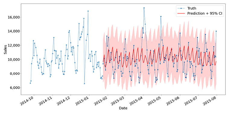
Figure 1.6: Forecasting store sales.

One issue here is that implementing a forecasting model like the one above for every store can quickly lead to hundreds or even thousands of models if the chain gathers enough data. Another issue is that not all stores are on the resource planning system used at the company yet, so some planners would like to retrieve forecasts for other stores they know are similar to their own. It is agreed that if users like this can explore regional profiles they believe are similar to their own data, then they can still make the optimal decisions.

Given this and the customer requirements for dynamic, ad hoc requests, you quickly rule out a full batch process. This wouldn’t cover the use case for regions not on the core system and wouldn’t allow for dynamic retrieval of up-to-date forecasts via the website, which would allow you to deploy models that forecast at a variety of time horizons in the future. It also means you could save on compute as you don’t need to manage the storage and updating of thousands of forecasts every day and your resources can be focused on model training.

Therefore, you decide that, actually, a web-hosted API with an endpoint that can return forecasts as needed by the user makes the most sense. To give efficient responses, you have to consider what happens in a typical user session. By workshopping with the potential users of the dashboard, you quickly realize that although the requests are dynamic, most planners will focus on particular items of interest in any one session. They will also not look at many regions. You then decide that it makes sense to have a caching strategy, where you take certain requests that you think might be common and cache them for reuse in the application.

This means that after the user makes their first selections, results can be returned more quickly for a better user experience. This leads to the rough system sketch in Figure 1.7:

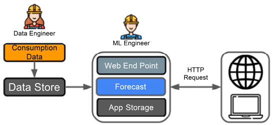
Figure 1.7: Example 2 workflow.

Next, let’s look at the final example.

Example 3: Classification pipeline

In this final example, you work for a web-based company that wants to classify users based on their usage patterns as targets for different types of advertising, in order to more effectively target marketing spend. For example, if the user uses the site less frequently, we may want to entice them with more aggressive discounts. One of the key requirements from the business is that the end results become part of the data landed in a data store used by other applications.

Based on these requirements, your team determines that a pipeline running a classification model is the simplest solution that ticks all the boxes. The data engineers focus their efforts on building the ingestion and data store infrastructure, while the ML engineer works to wrap up the classification model the data science team has trained on historical data. The base algorithm that the data scientists settle on is implemented in sklearn, which we will work through below by applying it to a marketing dataset that would be similar to that produced in this use case.

This hypothetical example aligns with a lot of classic datasets, including the Bank Marketing dataset from the UCI ML repository: https://archive.ics.uci.edu/ml/datasets/Bank+Marketing#. As in the previous example, there is a script you can run from the command line, this time in the Chapter01/classifying folder and called classify_example.py:

python3 classify_example.py

Running this script will read in the downloaded bank data, rebalance the training dataset, and then execute a hyperparameter optimization run on a randomized grid search for a random forest classifier. Similarly to before, we will show how these pieces work to give a flavor of how a data science team might have approached this problem:

1. The main block of the script contains all the relevant steps, which are neatly wrapped up into methods we will dissect over the next few steps:

   if __name__ == "__main__":
       X_train, X_test, y_train, y_test = ingest_and_prep_data()
       X_balanced, y_balanced = rebalance_classes(X_train, y_train)
       rf_random = get_randomised_rf_cv(
                     random_grid=get_hyperparam_grid()
                     )
       rf_random.fit(X_balanced, y_balanced)
   

2. The ingest_and_prep_data function is given below, and it does assume that the bank.csv data is stored in a directory called bank_data in the current folder. It reads the data into a pandas DataFrame, before performing a train-test split on the data and one-hot encoding the training features, before returning all the train and test features and targets. As in the other examples, most of these concepts and tools will be explained throughout the book, particularly in Chapter 3, From Model to Model Factory:

   def ingest_and_prep_data(
           bank_dataset: str = 'bank_data/bank.csv'
           ) -> tuple[pd.DataFrame, pd.DataFrame, pd.DataFrame,
                      pd.DataFrame]:
       df = pd.read_csv('bank_data/bank.csv', delimiter=';',
                         decimal=',')
       
       feature_cols = ['job', 'marital', 'education', 'contact',
                       'housing', 'loan', 'default', 'day']
       X = df[feature_cols].copy()
       y = df['y'].apply(lambda x: 1 if x == 'yes' else 0).copy()
       X_train, X_test, y_train, y_test = train_test_split(X, y, test_
                                             size=0.2, random_state=42)
       enc = OneHotEncoder(handle_unknown='ignore')
       X_train = enc.fit_transform(X_train)
       return X_train, X_test, y_train, y_test
   

3. Because the data is imbalanced, we need to rebalance the training data with an oversampling technique. In this example, we will use the Synthetic Minority Over-Sampling Technique (SMOTE) from the imblearn package:

   def rebalance_classes(X: pd.DataFrame, y: pd.DataFrame
                         ) -> tuple[pd.DataFrame, pd.DataFrame]:
       sm = SMOTE()
       X_balanced, y_balanced = sm.fit_resample(X, y)
       return X_balanced, y_balanced
   

4. Now we will move on to the main ML components of the script. We will perform a hyperparameter search (there’ll be more on this in Chapter 3, From Model to Model Factory), so we have to define a grid to search over:

   def get_hyperparam_grid() -> dict:
       n_estimators = [int(x) for x in np.linspace(start=200,
                       stop=2000, num=10)]
       max_features = ['auto', 'sqrt']
       max_depth = [int(x) for x in np.linspace(10, 110, num=11)]
       max_depth.append(None)
       min_samples_split = [2, 5, 10]
       min_samples_leaf = [1, 2, 4]
       bootstrap = [True, False]  # Create the random grid
       random_grid = {
           'n_estimators': n_estimators,
           'max_features': max_features,
           'max_depth': max_depth,
           'min_samples_split': min_samples_split,
           'min_samples_leaf': min_samples_leaf,
           'bootstrap': bootstrap
       }
       return random_grid
   

5. Then finally, this grid of hyperparameters will be used in the definition of a RandomisedSearchCV object that allows us to optimize an estimator (here, a RandomForestClassifier) over the hyperparameter values:

   def get_randomised_rf_cv(random_grid: dict) -> sklearn.model_
                                  selection._search.RandomizedSearchCV:
       rf = RandomForestClassifier()
       rf_random = RandomizedSearchCV(
           estimator=rf,
           param_distributions=random_grid,
           n_iter=100,
           cv=3,
           verbose=2,
           random_state=42,
           n_jobs=-1,
           scoring='f1'
       )
       return rf_random
   

The example above highlights the basic components of creating a typical classification model, but the question we have to ask ourselves as engineers is, “Then what?” It is clear that we have to actually run predictions with the model that has been produced, so we’ll need to persist it somewhere and read it in later. This is similar to the other use cases discussed in this chapter. Where things are more challenging here is that in this case, the engineers may actually consider not running in a batch or request-response scenario but in a streaming context. This means we will have to consider new technologies like Apache Kafka that enable you to both publish and subscribe to “topics” where packets of data called “events” can be shared. Not only that, but we will also have to make decisions about how to interact with data in this way using an ML model, raising questions about the appropriate model hosting mechanism. There will also be some subtleties around how often you want to retrain your algorithm to make sure that the classifier does not go stale. This is before we consider questions of latency or of monitoring the model’s performance in this very different setting. As you can see, this means that the ML engineer’s job here is quite a complex one. Figure 1.8 subsumes all this complexity into a very high-level diagram that would allow you to start considering the sort of system interactions you would need to build if you were the engineer on this project.

We will not cover streaming in that much detail in this book, but we will cover all of the other key components that would help you build out this example into a real solution in a lot of detail. For more details on streaming ML applications please see the book Machine Learning for Streaming Data with Python by Joose Korstanje, Packt, 2022.

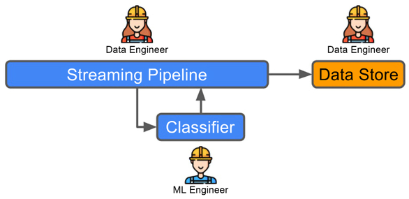
Figure 1.8: Example 3 workflow.

We have now explored three high-level ML system designs and discussed the rationale behind our workflow choices. We have also explored in detail the sort of code that would often be produced by data scientists working on modeling, but which would act as input to future ML engineering work. This section should, therefore, have given us an appreciation of where our engineering work begins in a typical project and what types of problems we aim to solve. And there you go. You are already on your way to becoming an ML engineer!