Search icon CANCEL
Subscription
0
Cart icon
Your Cart (0 item)
Close icon
You have no products in your basket yet
Save more on your purchases! discount-offer-chevron-icon
Savings automatically calculated. No voucher code required.
Arrow left icon
Explore Products
Best Sellers
New Releases
Books
Videos
Audiobooks
Learning Hub
Newsletter Hub
Free Learning
Arrow right icon
timer SALE ENDS IN
0 Days
:
00 Hours
:
00 Minutes
:
00 Seconds
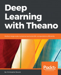
Deep Learning with Theano

Deep Learning with Theano: Perform large-scale numerical and scientific computations efficiently

eBook
$9.99 $39.99
Paperback
$48.99
Subscription
Free Trial
Renews at $19.99p/m

What do you get with eBook?

Product feature icon Instant access to your Digital eBook purchase
Product feature icon Download this book in EPUB and PDF formats
Product feature icon Access this title in our online reader with advanced features
Product feature icon DRM FREE - Read whenever, wherever and however you want
OR
Modal Close icon
Payment Processing...
tick Completed

Billing Address

Table of content icon View table of contents Preview book icon Preview Book

Deep Learning with Theano

Chapter 1. Theano Basics

This chapter presents Theano as a compute engine and the basics for symbolic computing with Theano. Symbolic computing consists of building graphs of operations that will be optimized later on for a specific architecture, using the computation libraries available for this architecture.

Although this chapter might appear to be a long way from practical applications, it is essential to have an understanding of the technology for the following chapters; what is it capable of and what value does it bring? All the following chapters address the applications of Theano when building all possible deep learning architectures.

Theano may be defined as a library for scientific computing; it has been available since 2007 and is particularly suited to deep learning. Two important features are at the core of any deep learning library: tensor operations, and the capability to run the code on CPU or Graphical Computation Unit (GPU). These two features enable us to work with a massive amount of multi-dimensional data. Moreover, Theano proposes automatic differentiation, a very useful feature that can solve a wider range of numeric optimizations than deep learning problems.

The chapter covers the following topics:

  • Theano installation and loading
  • Tensors and algebra
  • Symbolic programming
  • Graphs
  • Automatic differentiation
  • GPU programming
  • Profiling
  • Configuration

The need for tensors

Usually, input data is represented with multi-dimensional arrays:

  • Images have three dimensions: The number of channels, the width, and the height of the image
  • Sounds and times series have one dimension: The duration
  • Natural language sequences can be represented by two-dimensional arrays: The duration and the alphabet length or the vocabulary length

We'll see more examples of input data arrays in the future chapters.

In Theano, multi-dimensional arrays are implemented with an abstraction class, named tensor, with many more transformations available than traditional arrays in a computer language such as Python.

At each stage of a neural net, computations such as matrix multiplications involve multiple operations on these multi-dimensional arrays.

Classical arrays in programming languages do not have enough built-in functionalities to quickly and adequately address multi-dimensional computations and manipulations.

Computations on multi-dimensional arrays have a long history of optimizations, with tons of libraries and hardware. One of the most important gains in speed has been permitted by the massive parallel architecture of the GPU, with computation ability on a large number of cores, from a few hundred to a few thousand.

Compared to the traditional CPU, for example, a quadricore, 12-core, or 32-core engine, the gains with GPU can range from 5x to 100x, even if part of the code is still being executed on the CPU (data loading, GPU piloting, and result outputting). The main bottleneck with the use of GPU is usually the transfer of data between the memory of the CPU and the memory of the GPU, but still, when well programmed, the use of GPU helps bring a significant increase in speed of an order of magnitude. Getting results in days rather than months, or hours rather than days, is an undeniable benefit for experimentation.

The Theano engine has been designed to address the challenges of multi-dimensional arrays and architecture abstraction from the beginning.

There is another undeniable benefit of Theano for scientific computation: the automatic differentiation of functions of multi-dimensional arrays, a well-suited feature for model parameter inference via objective function minimization. Such a feature facilitates experimentation by releasing the pain to compute derivatives, which might not be very complicated, but are prone to many errors.

Installing and loading Theano

In this section, we'll install Theano, run it on the CPU and GPU devices, and save the configuration.

Conda package and environment manager

The easiest way to install Theano is to use conda, a cross-platform package and environment manager.

If conda is not already installed on your operating system, the fastest way to install conda is to download the miniconda installer from https://conda.io/miniconda.html. For example, for conda under Linux 64 bit and Python 2.7, use this command:

wget https://repo.continuum.io/miniconda/Miniconda2-latest-Linux-x86_64.sh
chmod +x Miniconda2-latest-Linux-x86_64.sh
bash ./Miniconda2-latest-Linux-x86_64.sh

Conda enables us to create new environments in which versions of Python (2 or 3) and the installed packages may differ. The conda root environment uses the same version of Python as the version installed on the system on which you installed conda.

Installing and running Theano on CPU

Let's install Theano:

conda install theano

Run a Python session and try the following commands to check your configuration:

>>> from theano import theano

>>> theano.config.device
'cpu'

>>> theano.config.floatX
'float64'

>>> print(theano.config)

The last command prints all the configuration of Theano. The theano.config object contains keys to many configuration options.

To infer the configuration options, Theano looks first at the ~/.theanorc file, then at any environment variables that are available, which override the former options, and lastly at the variable set in the code that are first in order of precedence:

>>> theano.config.floatX='float32'

Some of the properties might be read-only and cannot be changed in the code, but floatX, which sets the default floating point precision for floats, is among the properties that can be changed directly in the code.

Note

It is advised to use float32 since GPU has a long history without float64. float64 execution speed on GPU is slower, sometimes much slower (2x to 32x on latest generation Pascal hardware), and float32 precision is enough in practice.

GPU drivers and libraries

Theano enables the use of GPU, units that are usually used to compute the graphics to display on the computer screen.

To have Theano work on the GPU as well, a GPU backend library is required on your system.

The CUDA library (for NVIDIA GPU cards only) is the main choice for GPU computations. There is also the OpenCL standard, which is open source but far less developed, and much more experimental and rudimentary on Theano.

Most scientific computations still occur on NVIDIA cards at the moment. If you have an NVIDIA GPU card, download CUDA from the NVIDIA website, https://developer.nvidia.com/cuda-downloads, and install it. The installer will install the latest version of the GPU drivers first, if they are not already installed. It will install the CUDA library in the /usr/local/cuda directory.

Install the cuDNN library, a library by NVIDIA, that offers faster implementations of some operations for the GPU. To install it, I usually copy the /usr/local/cuda directory to a new directory, /usr/local/cuda-{CUDA_VERSION}-cudnn-{CUDNN_VERSION}, so that I can choose the version of CUDA and cuDNN, depending on the deep learning technology I use and its compatibility.

In your .bashrc profile, add the following line to set the $PATH and $LD_LIBRARY_PATH variables:

export PATH=/usr/local/cuda-8.0-cudnn-5.1/bin:$PATH
export LD_LIBRARY_PATH=/usr/local/cuda-8.0-cudnn-5.1/lib64:/usr/local/cuda-8.0-cudnn-5.1/lib:$LD_LIBRARY_PATH

Installing and running Theano on GPU

N-dimensional GPU arrays have been implemented in Python in six different GPU libraries (Theano/CudaNdarray,PyCUDA/ GPUArray,CUDAMAT/ CUDAMatrix, PYOPENCL/GPUArray, Clyther, Copperhead), are a subset of NumPy.ndarray. Libgpuarray is a backend library to have them in a common interface with the same property.

To install libgpuarray with conda, use this command:

conda install pygpu

To run Theano in GPU mode, you need to configure the config.device variable before execution since it is a read-only variable once the code is run. Run this command with the THEANO_FLAGS environment variable:

THEANO_FLAGS="device=cuda,floatX=float32" python
>>> import theano
Using cuDNN version 5110 on context None
Mapped name None to device cuda: Tesla K80 (0000:83:00.0)

>>> theano.config.device
'gpu'

>>> theano.config.floatX
'float32'

The first return shows that GPU device has been correctly detected, and specifies which GPU it uses.

By default, Theano activates CNMeM, a faster CUDA memory allocator. An initial pre-allocation can be specified with the gpuarra.preallocate option. At the end, my launch command will be as follows:

THEANO_FLAGS="device=cuda,floatX=float32,gpuarray.preallocate=0.8" python
>>> from theano import theano
Using cuDNN version 5110 on context None
Preallocating 9151/11439 Mb (0.800000) on cuda
Mapped name None to device cuda: Tesla K80 (0000:83:00.0)

The first line confirms that cuDNN is active, the second confirms memory pre-allocation. The third line gives the default context name (that is, None when flag device=cuda is set) and the model of GPU used, while the default context name for the CPU will always be cpu.

It is possible to specify a different GPU than the first one, setting the device to cuda0, cuda1,... for multi-GPU computers. It is also possible to run a program on multiple GPU in parallel or in sequence (when the memory of one GPU is not sufficient), in particular when training very deep neural nets, as for classification of full images as described in Chapter 7, Classifying Images with Residual Networks. In this case, the contexts=dev0->cuda0;dev1->cuda1;dev2->cuda2;dev3->cuda3 flag activates multiple GPUs instead of one, and designates the context name to each GPU device to be used in the code. Here is an example on a 4-GPU instance:

THEANO_FLAGS="contexts=dev0->cuda0;dev1->cuda1;dev2->cuda2;dev3->cuda3,floatX=float32,gpuarray.preallocate=0.8" python
>>> import theano
Using cuDNN version 5110 on context None
Preallocating 9177/11471 Mb (0.800000) on cuda0
Mapped name dev0 to device cuda0: Tesla K80 (0000:83:00.0)
Using cuDNN version 5110 on context dev1
Preallocating 9177/11471 Mb (0.800000) on cuda1
Mapped name dev1 to device cuda1: Tesla K80 (0000:84:00.0)
Using cuDNN version 5110 on context dev2
Preallocating 9177/11471 Mb (0.800000) on cuda2
Mapped name dev2 to device cuda2: Tesla K80 (0000:87:00.0)
Using cuDNN version 5110 on context dev3
Preallocating 9177/11471 Mb (0.800000) on cuda3
Mapped name dev3 to device cuda3: Tesla K80 (0000:88:00.0)

To assign computations to a specific GPU in this multi-GPU setting, the names we choose, dev0, dev1, dev2, and dev3, have been mapped to each device (cuda0, cuda1, cuda2, cuda3).

This name mapping enables to write codes that are independent of the underlying GPU assignments and libraries (CUDA or others).

To keep the current configuration flags active at every Python session or execution without using environment variables, save your configuration in the ~/.theanorc file as follows:

 [global]
 floatX = float32
 device = cuda0
 [gpuarray]
 preallocate = 1

Now you can simply run python command. You are now all set.

Tensors

In Python, some scientific libraries such as NumPy provide multi-dimensional arrays. Theano doesn't replace Numpy, but it works in concert with it. NumPy is used for the initialization of tensors.

To perform the same computation on CPU and GPU, variables are symbolic and represented by the tensor class, an abstraction, and writing numerical expressions consists of building a computation graph of variable nodes and apply nodes. Depending on the platform on which the computation graph will be compiled, tensors are replaced by either of the following:

  • A TensorType variable, which has to be on CPU
  • A GpuArrayType variable, which has to be on GPU

That way, the code can be written indifferently of the platform where it will be executed.

Here are a few tensor objects:

Object class

Number of dimensions

Example

theano.tensor.scalar

0-dimensional array

1, 2.5

theano.tensor.vector

1-dimensional array

[0,3,20]

theano.tensor.matrix

2-dimensional array

[[2,3][1,5]]

theano.tensor.tensor3

3-dimensional array

[[[2,3][1,5]],[[1,2],[3,4]]]

Playing with these Theano objects in the Python shell gives us a better idea:

>>> import theano.tensor as T

>>> T.scalar()
<TensorType(float32, scalar)>

>>> T.iscalar()
<TensorType(int32, scalar)>

>>> T.fscalar()
<TensorType(float32, scalar)>

>>> T.dscalar()
<TensorType(float64, scalar)>

With i, l, f, or d in front of the object name, you initiate a tensor of a given type, integer32, integer64, float32, or float64. For real-valued (floating point) data, it is advised to use the direct form T.scalar() instead of the f or d variants since the direct form will use your current configuration for floats:

>>> theano.config.floatX = 'float64'

>>> T.scalar()
<TensorType(float64, scalar)>

>>> T.fscalar()
<TensorType(float32, scalar)>

>>> theano.config.floatX = 'float32'

>>> T.scalar()
<TensorType(float32, scalar)>

Symbolic variables do either of the following:

  • Play the role of placeholders, as a starting point to build your graph of numerical operations (such as addition, multiplication): they receive the flow of the incoming data during the evaluation once the graph has been compiled
  • Represent intermediate or output results

Symbolic variables and operations are both part of a computation graph that will be compiled either on CPU or GPU for fast execution. Let's write our first computation graph consisting of a simple addition:

>>> x = T.matrix('x')

>>> y = T.matrix('y')

>>> z = x + y

>>> theano.pp(z)
'(x + y)'

>>> z.eval({x: [[1, 2], [1, 3]], y: [[1, 0], [3, 4]]})
array([[ 2.,  2.],
       [ 4.,  7.]], dtype=float32)

First, two symbolic variables, or variable nodes, are created, with the names x and y, and an addition operation, an apply node, is applied between both of them to create a new symbolic variable, z, in the computation graph.

The pretty print function, pp, prints the expression represented by Theano symbolic variables. Eval evaluates the value of the output variable, z, when the first two variables, x and y, are initialized with two numerical 2-dimensional arrays.

The following example shows the difference between the variables x and y, and their names x and y:

>>> a = T.matrix()

>>> b = T.matrix()

>>> theano.pp(a + b)
'(<TensorType(float32, matrix)> + <TensorType(float32, matrix)>)'.

Without names, it is more complicated to trace the nodes in a large graph. When printing the computation graph, names significantly help diagnose problems, while variables are only used to handle the objects in the graph:

>>> x = T.matrix('x')

>>> x = x + x

>>> theano.pp(x)
'(x + x)'

Here, the original symbolic variable, named x, does not change and stays part of the computation graph. x + x creates a new symbolic variable we assign to the Python variable x.

Note also that with the names, the plural form initializes multiple tensors at the same time:

>>> x, y, z = T.matrices('x', 'y', 'z')

Now, let's have a look at the different functions to display the graph.

Graphs and symbolic computing

Let's take back the simple addition example and present different ways to display the same information:

>>> x = T.matrix('x')

>>> y = T.matrix('y')

>>> z = x + y

>>> z

Elemwise{add,no_inplace}.0

>>> theano.pp(z)

'(x + y)

>>> theano.printing.pprint(z)

'(x + y)'

>>> theano.printing.debugprint(z)
Elemwise{add,no_inplace} [id A] ''   
 |x [id B]
 |y [id C]

Here, the debugprint function prints the pre-compilation graph, the unoptimized graph. In this case, it is composed of two variable nodes, x and y, and an apply node, the elementwise addition, with the no_inplace option. The inplace option will be used in the optimized graph to save memory and re-use the memory of the input to store the result of the operation.

If the graphviz and pydot libraries have been installed, the pydotprint command outputs a PNG image of the graph:

>>> theano.printing.pydotprint(z)
The output file is available at ~/.theano/compiledir_Linux-4.4--generic-x86_64-with-Ubuntu-16.04-xenial-x86_64-2.7.12-64/theano.pydotprint.gpu.png.
Graphs and symbolic computing

You might have noticed that the z.eval command takes while to execute the first time. The reason for this delay is the time required to optimize the mathematical expression and compile the code for the CPU or GPU before being evaluated.

The compiled expression can be obtained explicitly and used as a function that behaves as a traditional Python function:

>>> addition = theano.function([x, y], [z])

>>> addition([[1, 2], [1, 3]], [[1, 0], [3, 4]])
[array([[ 2.,  2.],
       [ 4.,  7.]], dtype=float32)]

The first argument in the function creation is a list of variables representing the input nodes of the graph. The second argument is the array of output variables. To print the post compilation graph, use this command:

>>> theano.printing.debugprint(addition)
HostFromGpu(gpuarray) [id A] ''   3
 |GpuElemwise{Add}[(0, 0)]<gpuarray> [id B] ''   2
   |GpuFromHost<None> [id C] ''   1
   | |x [id D]
   |GpuFromHost<None> [id E] ''   0
     |y [id F]

>>> theano.printing.pydotprint(addition)

The output file is available at ~/.theano/compiledir_Linux-4.4--generic-x86_64-with-Ubuntu-16.04-xenial-x86_64-2.7.12-64/theano.pydotprint.gpu.png:
Graphs and symbolic computing

This case has been printed while using the GPU. During compilation, each operation has chosen the available GPU implementation. The main program still runs on CPU, where the data resides, but a GpuFromHost instruction performs a data transfer from the CPU to the GPU for input, while the opposite operation, HostFromGpu, fetches the result for the main program to display it:

Graphs and symbolic computing

Theano performs some mathematical optimizations, such as grouping elementwise operations, adding a new value to the previous addition:

>>> z= z * x

>>> theano.printing.debugprint(theano.function([x,y],z))
HostFromGpu(gpuarray) [id A] ''   3
 |GpuElemwise{Composite{((i0 + i1) * i0)}}[(0, 0)]<gpuarray> [id B] ''   2
   |GpuFromHost<None> [id C] ''   1
   | |x [id D]
   |GpuFromHost<None> [id E] ''   0
     |y [id F]

The number of nodes in the graph has not increased: two additions have been merged into one node. Such optimizations make it more tricky to debug, so we'll show you at the end of this chapter how to disable optimizations for debugging.

Lastly, let's see a bit more about setting the initial value with NumPy:

>>> theano.config.floatX
'float32'

>>> x = T.matrix()

>>> x
<TensorType(float32, matrix)>

>>> y = T.matrix()

>>> addition = theano.function([x, y], [x+y])

>>> addition(numpy.ones((2,2)),numpy.zeros((2,2)))
Traceback (most recent call last):
  File "<stdin>", line 1, in <module>
  File "/usr/local/lib/python2.7/site-packages/theano/compile/function_module.py", line 786, in __call__
    allow_downcast=s.allow_downcast)

  File "/usr/local/lib/python2.7/site-packages/theano/tensor/type.py", line 139, in filter
    raise TypeError(err_msg, data)
TypeError: ('Bad input argument to theano function with name "<stdin>:1"  at index 0(0-based)', 'TensorType(float32, matrix) cannot store a value of dtype float64 without risking loss of precision. If you do not mind this loss, you can: 1) explicitly cast your data to float32, or 2) set "allow_input_downcast=True" when calling "function".', array([[ 1.,  1.],
       [ 1.,  1.]]))

Executing the function on the NumPy arrays throws an error related to loss of precision, since the NumPy arrays here have float64 and int64 dtypes, but x and y are float32. There are multiple solutions to this; the first is to create the NumPy arrays with the right dtype:

>>> import numpy

>>> addition(numpy.ones((2,2), dtype=theano.config.floatX),numpy.zeros((2,2), dtype=theano.config.floatX))
[array([[ 1.,  1.],
        [ 1.,  1.]], dtype=float32)]

Alternatively, cast the NumPy arrays (in particular for numpy.diag, which does not allow us to choose the dtype directly):

>>> addition(numpy.ones((2,2)).astype(theano.config.floatX),numpy.diag((2,3)).astype(theano.config.floatX))
[array([[ 3.,  1.],
        [ 1.,  4.]], dtype=float32)]

Or we could allow downcasting:

>>> addition = theano.function([x, y], [x+y],allow_input_downcast=True)

>>> addition(numpy.ones((2,2)),numpy.zeros((2,2)))
[array([[ 1.,  1.],
        [ 1.,  1.]], dtype=float32)]

Operations on tensors

We have seen how to create a computation graph composed of symbolic variables and operations, and compile the resulting expression for an evaluation or as a function, either on GPU or on CPU.

As tensors are very important to deep learning, Theano provides lots of operators to work with tensors. Most operators that exist in scientific computing libraries such as NumPy for numerical arrays have their equivalent in Theano and have a similar name, in order to be more familiar to NumPy's users. But contrary to NumPy, expressions written with Theano can be compiled either on CPU or GPU.

This, for example, is the case for tensor creation:

  • T.zeros(), T.ones(), T.eye() operators take a shape tuple as input
  • T.zeros_like(), T.one_like(), T.identity_like() use the shape of the tensor argument
  • T.arange(), T.mgrid(), T.ogrid() are used for range and mesh grid arrays

Let's have a look in the Python shell:

>>> a = T.zeros((2,3))

>>> a.eval()
array([[ 0.,  0.,  0.],
       [ 0.,  0.,  0.]])

>>> b = T.identity_like(a)

>>> b.eval()
array([[ 1.,  0.,  0.],
        [ 0.,  1.,  0.]])

>>> c = T.arange(10)

>>> c.eval()
array([0, 1, 2, 3, 4, 5, 6, 7, 8, 9])

Information such as the number of dimensions, ndim, and the type, dtype, are defined at tensor creation and cannot be modified later:

>>> c.ndim
1

>>> c.dtype
'int64'

>>> c.type
TensorType(int64, vector)

Some other information, such as shape, is evaluated by the computation graph:

>>> a = T.matrix()

>>> a.shape
Shape.0

>>> a.shape.eval({a: [[1, 2], [1, 3]]})
array([2, 2])

>>> shape_fct = theano.function([a],a.shape)

>>> shape_fct([[1, 2], [1, 3]])
array([2, 2])

>>> n = T.iscalar()

>>> c = T.arange(n)

>>> c.shape.eval({n:10})
array([10])

Dimension manipulation operators

The first type of operator on tensor is for dimension manipulation. This type of operator takes a tensor as input and returns a new tensor:

Operator

Description

T.reshape

Reshape the dimension of the tensor

T.fill

Fill the array with the same value

T.flatten

Return all elements in a 1-dimensional tensor (vector)

T.dimshuffle

Change the order of the dimension, more or less like NumPy's transpose method – the main difference is that it can be used to add or remove broadcastable dimensions (of length 1).

T.squeeze

Reshape by removing dimensions equal to 1

T.transpose

Transpose

T.swapaxes

Swap dimensions

T.sort, T.argsort

Sort tensor, or indices of the order

For example, the reshape operation's output represents a new tensor, containing the same elements in the same order but in a different shape:

>>> a = T.arange(10)

>>> b = T.reshape( a, (5,2) )

>>> b.eval()
array([[0, 1],
       [2, 3], 
       [4, 5],
       [6, 7],
       [8, 9]])

The operators can be chained:

>>> T.arange(10).reshape((5,2))[::-1].T.eval()
array([[8, 6, 4, 2, 0],
       [9, 7, 5, 3, 1]])

Notice the use of traditional [::-1] array access by indices in Python and the .T for T.transpose.

Elementwise operators

The second type of operations on multi-dimensional arrays is elementwise operators.

The first category of elementwise operations takes two input tensors of the same dimensions and applies a function, f, elementwise, which means on all pairs of elements with the same coordinates in the respective tensors f([a,b],[c,d]) = [ f(a,c), f(b,d)]. For example, here's multiplication:

>>> a, b = T.matrices('a', 'b')

>>> z = a * b

>>> z.eval({a:numpy.ones((2,2)).astype(theano.config.floatX), b:numpy.diag((3,3)).astype(theano.config.floatX)})
array([[ 3.,  0.],
       [ 0.,  3.]])

The same multiplication can be written as follows:

>>> z = T.mul(a, b)

T.add and T.mul accept an arbitrary number of inputs:

>>> z = T.mul(a, b, a, b)

Some elementwise operators accept only one input tensor f([a,b]) = [f(a),f(b)]):

>>> a = T.matrix()

>>> z = a ** 2 

>>> z.eval({a:numpy.diag((3,3)).astype(theano.config.floatX)})
array([[ 9.,  0.], 
       [ 0.,  9.]])

Lastly, I would like to introduce the mechanism of broadcasting. When the input tensors do not have the same number of dimensions, the missing dimension will be broadcasted, meaning the tensor will be repeated along that dimension to match the dimension of the other tensor. For example, taking one multi-dimensional tensor and a scalar (0-dimensional) tensor, the scalar will be repeated in an array of the same shape as the multi-dimensional tensor so that the final shapes will match and the elementwise operation will be applied, f([a,b], c) = [ f(a,c), f(b,c) ]:

>>> a = T.matrix()

>>> b = T.scalar()

>>> z = a * b

>>> z.eval({a:numpy.diag((3,3)).astype(theano.config.floatX),b:3})
array([[ 6.,  0.],
       [ 0.,  6.]])

Here is a list of elementwise operations:

Operator

Other form

Description

T.add, T.sub, T.mul, T.truediv

+, -, *, /

Add, subtract, multiply, divide

T.pow, T.sqrt

**, T.sqrt

Power, square root

T.exp, T.log


Exponential, logarithm

T.cos, T.sin, T.tan


Cosine, sine, tangent

T.cosh, T.sinh, T.tanh


Hyperbolic trigonometric functions

T.intdiv, T.mod

//, %

Int div, modulus

T.floor, T.ceil, T.round


Rounding operators

T.sgn


Sign

T.and_, T.xor, T.or_, T.invert

&,^,|,~

Bitwise operators

T.gt, T.lt, T.ge, T.le

>, <, >=, <=

Comparison operators

T.eq, T.neq, T.isclose


Equality, inequality, or close with tolerance

T.isnan


Comparison with NaN (not a number)

T.abs_


Absolute value

T.minimum, T.maximum


Minimum and maximum elementwise

T.clip


Clip the values between a maximum and a minimum

T.switch


Switch

T.cast


Tensor type casting

The elementwise operators always return an array with the same size as the input array. T.switch and T.clip accept three inputs.

In particular, T.switch will perform the traditional switch operator elementwise:

>>> cond = T.vector('cond')

>>> x,y = T.vectors('x','y')

>>> z = T.switch(cond, x, y)

>>> z.eval({ cond:[1,0], x:[10,10], y:[3,2] })
array([ 10.,   2.], dtype=float32)

At the same position where cond tensor is true, the result has the x value; otherwise, if it is false, it has the y value.

For the T.switch operator, there is a specific equivalent, ifelse, that takes a scalar condition instead of a tensor condition. It is not an elementwise operation though, and supports lazy evaluation (not all elements are computed if the answer is known before it finishes):

>>> from theano.ifelse import ifelse

>>> z=ifelse(1, 5, 4)

>>> z.eval()
array(5, dtype=int8)

Reduction operators

Another type of operation on tensors is reductions, reducing all elements to a scalar value in most cases, and for that purpose, it is required to scan all the elements of the tensor to compute the output:

Operator

Description

T.max, T.argmax, T.max_and_argmax

Maximum, index of the maximum

T.min, T.argmin

Minimum, index of the minimum

T.sum, T.prod

Sum or product of elements

T.mean, T.var, T.std

Mean, variance, and standard deviation

T.all, T.any

AND and OR operations with all elements

T.ptp

Range of elements (minimum, maximum)

These operations are also available row-wise or column-wise by specifying an axis and the dimension along which the reduction is performed:

>>> a = T.matrix('a')

>>> T.max(a).eval({a:[[1,2],[3,4]]})
array(4.0, dtype=float32)

>>> T.max(a,axis=0).eval({a:[[1,2],[3,4]]})
array([ 3.,  4.], dtype=float32)

>>> T.max(a,axis=1).eval({a:[[1,2],[3,4]]})
array([ 2.,  4.], dtype=float32)

Linear algebra operators

A third category of operations are the linear algebra operators, such as matrix multiplication:

Linear algebra operators

Also called inner product for vectors:

Linear algebra operators

Operator

Description

T.dot

Matrix multiplication/inner product

T.outer

Outer product

There are some generalized (T.tensordot to specify the axis), or batched (batched_dot, batched_tensordot) versions of the operators.

Lastly, a few operators remain and can be very useful, but they do not belong to any of the previous categories: T.concatenate concatenates the tensors along the specified dimension, T.stack creates a new dimension to stack the input tensors, and T.stacklist creates new patterns to stack tensors together:

>>> a = T.arange(10).reshape((5,2))

>>> b = a[::-1]

>>> b.eval()
array([[8, 9],
       [6, 7],
       [4, 5],
       [2, 3],
       [0, 1]])
>>> a.eval()
array([[0, 1],
       [2, 3],
       [4, 5],
       [6, 7],
       [8, 9]])
>>> T.concatenate([a,b]).eval()
array([[0, 1],
       [2, 3],
       [4, 5],
       [6, 7],
       [8, 9],
       [8, 9],
       [6, 7],
       [4, 5],
       [2, 3],
       [0, 1]])
>>> T.concatenate([a,b],axis=1).eval()
array([[0, 1, 8, 9],
       [2, 3, 6, 7],
       [4, 5, 4, 5],
       [6, 7, 2, 3],
       [8, 9, 0, 1]])

>>> T.stack([a,b]).eval()
array([[[0, 1],
        [2, 3],
        [4, 5],
        [6, 7],
        [8, 9]],
       [[8, 9],
        [6, 7],
        [4, 5],
        [2, 3],
        [0, 1]]])

An equivalent of the NumPy expressions a[5:] = 5 and a[5:] += 5 exists as two functions:

>>> a.eval()
array([[0, 1],
       [2, 3],
       [4, 5],
       [6, 7],
       [8, 9]])

>>> T.set_subtensor(a[3:], [-1,-1]).eval()

array([[ 0,  1],
       [ 2,  3],
       [ 4,  5],
       [-1, -1],
       [-1, -1]])

>>> T.inc_subtensor(a[3:], [-1,-1]).eval()
array([[0, 1],
       [2, 3],
       [4, 5],
       [5, 6],
       [7, 8]])

Unlike NumPy's syntax, the original tensor is not modified; instead, a new variable is created that represents the result of that modification. Therefore, the original variable a still refers to the original value, and the returned variable (here unassigned) represents the updated one, and the user should use that new variable in the rest of their computation.

Left arrow icon Right arrow icon
Download code icon Download Code

Key benefits

  • Learn Theano basics and evaluate your mathematical expressions faster and in an efficient manner
  • Learn the design patterns of deep neural architectures to build efficient and powerful networks on your datasets
  • Apply your knowledge to concrete fields such as image classification, object detection, chatbots, machine translation, reinforcement agents, or generative models.

Description

This book offers a complete overview of Deep Learning with Theano, a Python-based library that makes optimizing numerical expressions and deep learning models easy on CPU or GPU. The book provides some practical code examples that help the beginner understand how easy it is to build complex neural networks, while more experimented data scientists will appreciate the reach of the book, addressing supervised and unsupervised learning, generative models, reinforcement learning in the fields of image recognition, natural language processing, or game strategy. The book also discusses image recognition tasks that range from simple digit recognition, image classification, object localization, image segmentation, to image captioning. Natural language processing examples include text generation, chatbots, machine translation, and question answering. The last example deals with generating random data that looks real and solving games such as in the Open-AI gym. At the end, this book sums up the best -performing nets for each task. While early research results were based on deep stacks of neural layers, in particular, convolutional layers, the book presents the principles that improved the efficiency of these architectures, in order to help the reader build new custom nets.

Who is this book for?

This book is indented to provide a full overview of deep learning. From the beginner in deep learning and artificial intelligence, to the data scientist who wants to become familiar with Theano and its supporting libraries, or have an extended understanding of deep neural nets. Some basic skills in Python programming and computer science will help, as well as skills in elementary algebra and calculus.

What you will learn

  • Get familiar with Theano and deep learning
  • Provide examples in supervised, unsupervised, generative, or reinforcement learning.
  • Discover the main principles for designing efficient deep learning nets: convolutions, residual connections, and recurrent connections.
  • Use Theano on real-world computer vision datasets, such as for digit classification and image classification.
  • Extend the use of Theano to natural language processing tasks, for chatbots or machine translation
  • Cover artificial intelligence-driven strategies to enable a robot to solve games or learn from an environment
  • Generate synthetic data that looks real with generative modeling
  • Become familiar with Lasagne and Keras, two frameworks built on top of Theano

Product Details

Country selected
Publication date, Length, Edition, Language, ISBN-13
Publication date : Jul 31, 2017
Length: 300 pages
Edition : 1st
Language : English
ISBN-13 : 9781786463050
Vendor :
Google
Category :
Concepts :
Tools :

What do you get with eBook?

Product feature icon Instant access to your Digital eBook purchase
Product feature icon Download this book in EPUB and PDF formats
Product feature icon Access this title in our online reader with advanced features
Product feature icon DRM FREE - Read whenever, wherever and however you want
OR
Modal Close icon
Payment Processing...
tick Completed

Billing Address

Product Details

Publication date : Jul 31, 2017
Length: 300 pages
Edition : 1st
Language : English
ISBN-13 : 9781786463050
Vendor :
Google
Category :
Concepts :
Tools :

Packt Subscriptions

See our plans and pricing
Modal Close icon
$19.99 billed monthly
Feature tick icon Unlimited access to Packt's library of 7,000+ practical books and videos
Feature tick icon Constantly refreshed with 50+ new titles a month
Feature tick icon Exclusive Early access to books as they're written
Feature tick icon Solve problems while you work with advanced search and reference features
Feature tick icon Offline reading on the mobile app
Feature tick icon Simple pricing, no contract
$199.99 billed annually
Feature tick icon Unlimited access to Packt's library of 7,000+ practical books and videos
Feature tick icon Constantly refreshed with 50+ new titles a month
Feature tick icon Exclusive Early access to books as they're written
Feature tick icon Solve problems while you work with advanced search and reference features
Feature tick icon Offline reading on the mobile app
Feature tick icon Choose a DRM-free eBook or Video every month to keep
Feature tick icon PLUS own as many other DRM-free eBooks or Videos as you like for just $5 each
Feature tick icon Exclusive print discounts
$279.99 billed in 18 months
Feature tick icon Unlimited access to Packt's library of 7,000+ practical books and videos
Feature tick icon Constantly refreshed with 50+ new titles a month
Feature tick icon Exclusive Early access to books as they're written
Feature tick icon Solve problems while you work with advanced search and reference features
Feature tick icon Offline reading on the mobile app
Feature tick icon Choose a DRM-free eBook or Video every month to keep
Feature tick icon PLUS own as many other DRM-free eBooks or Videos as you like for just $5 each
Feature tick icon Exclusive print discounts

Frequently bought together


Stars icon
Total $29.97 $131.97 $102.00 saved
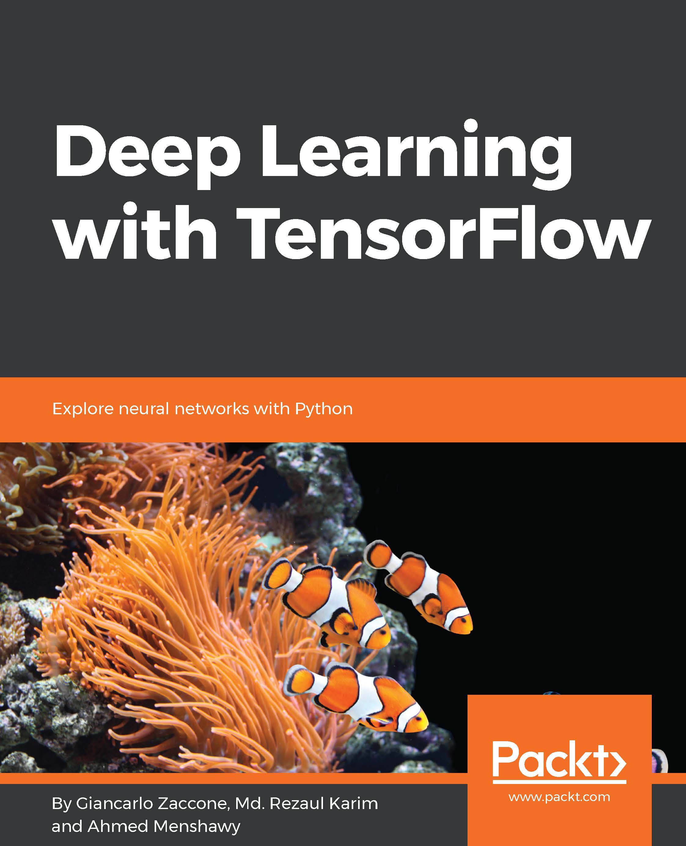
Deep Learning with TensorFlow
$54.99
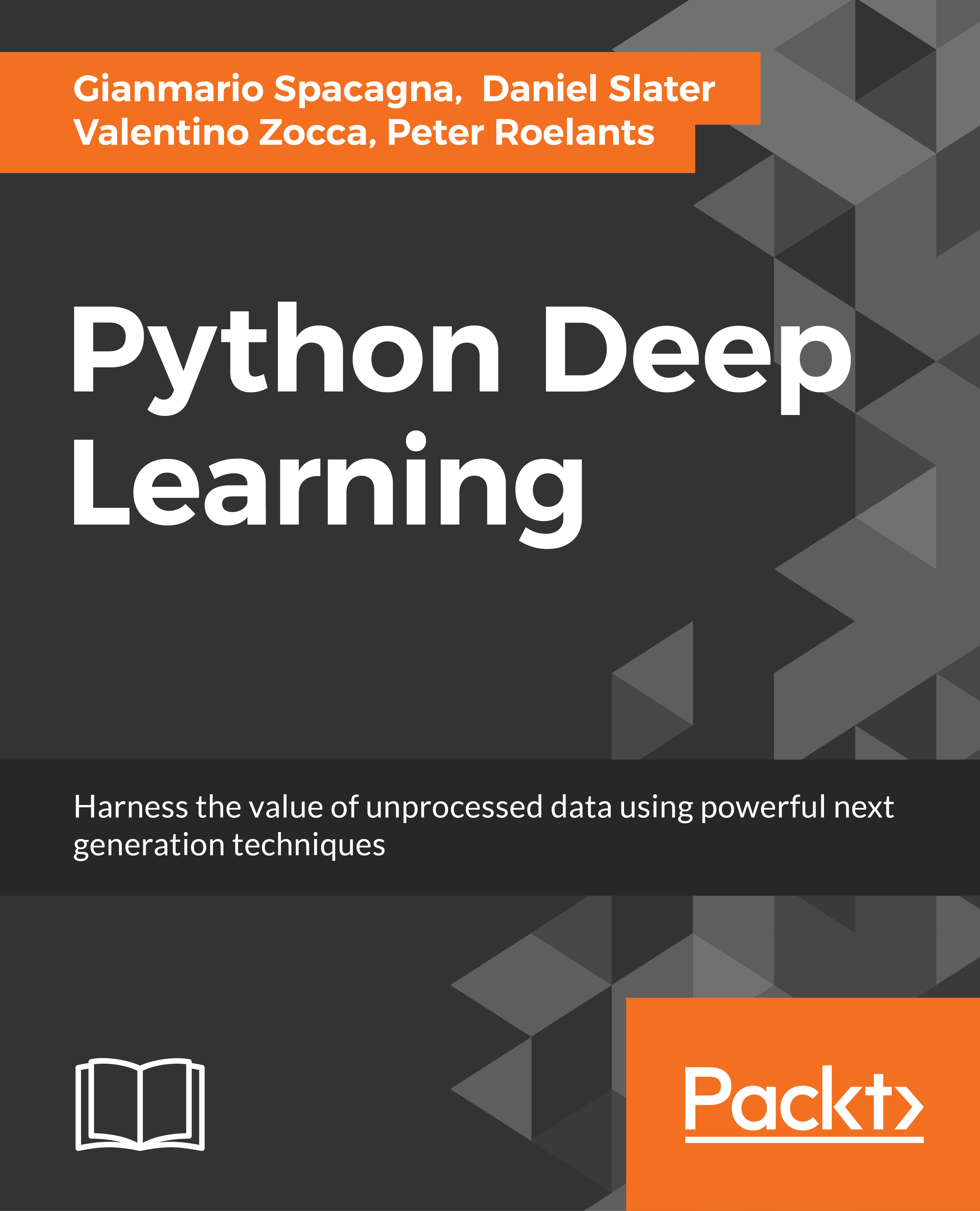
Python Deep Learning
$60.99
Deep Learning with Theano
$48.99
Total $29.97$131.97 $102.00 saved Stars icon
Banner background image

Table of Contents

14 Chapters
1. Theano Basics Chevron down icon Chevron up icon
2. Classifying Handwritten Digits with a Feedforward Network Chevron down icon Chevron up icon
3. Encoding Word into Vector Chevron down icon Chevron up icon
4. Generating Text with a Recurrent Neural Net Chevron down icon Chevron up icon
5. Analyzing Sentiment with a Bidirectional LSTM Chevron down icon Chevron up icon
6. Locating with Spatial Transformer Networks Chevron down icon Chevron up icon
7. Classifying Images with Residual Networks Chevron down icon Chevron up icon
8. Translating and Explaining with Encoding – decoding Networks Chevron down icon Chevron up icon
9. Selecting Relevant Inputs or Memories with the Mechanism of Attention Chevron down icon Chevron up icon
10. Predicting Times Sequences with Advanced RNN Chevron down icon Chevron up icon
11. Learning from the Environment with Reinforcement Chevron down icon Chevron up icon
12. Learning Features with Unsupervised Generative Networks Chevron down icon Chevron up icon
13. Extending Deep Learning with Theano Chevron down icon Chevron up icon
Index Chevron down icon Chevron up icon

Customer reviews

Rating distribution
Full star icon Full star icon Full star icon Half star icon Empty star icon 3.7
(3 Ratings)
5 star 66.7%
4 star 0%
3 star 0%
2 star 0%
1 star 33.3%
Coquard Aurélien Oct 10, 2017
Full star icon Full star icon Full star icon Full star icon Full star icon 5
Don't know where to start with Neural Networks and Deep Learning? Well, here is a perfect starting point, and more ... The walkthrough all Theano concepts is illustrated with really relevant examples and algorithms. Great book! Every student in the domain should have it.
Amazon Verified review Amazon
David Oct 08, 2017
Full star icon Full star icon Full star icon Full star icon Full star icon 5
The dean from my data science graduate program told me about this book, as I am huge fan of PackT publishing. This book provides excellent resources for implementing deep learning algorithms using the Theano library in python. Plus, at the end of each chapter the author has taken the extra step of listing resent articles and publications that are relevant to that particular area of deep learning in each chapter. This one has everything that I needed to prepare to execute a deep learning computer program. It is a great resource, and so far outside of just the technical guide for Theano, there is no other book like it.
Amazon Verified review Amazon
Maciek Aug 03, 2018
Full star icon Empty star icon Empty star icon Empty star icon Empty star icon 1
This book is horrible even by Packt standards. It's full of errors, it's poorly written to the point of being barely comprehensible in some places. It almost feels like this text has been generated by a neural network rather than being written by a human author.
Amazon Verified review Amazon
Get free access to Packt library with over 7500+ books and video courses for 7 days!
Start Free Trial

FAQs

How do I buy and download an eBook? Chevron down icon Chevron up icon

Where there is an eBook version of a title available, you can buy it from the book details for that title. Add either the standalone eBook or the eBook and print book bundle to your shopping cart. Your eBook will show in your cart as a product on its own. After completing checkout and payment in the normal way, you will receive your receipt on the screen containing a link to a personalised PDF download file. This link will remain active for 30 days. You can download backup copies of the file by logging in to your account at any time.

If you already have Adobe reader installed, then clicking on the link will download and open the PDF file directly. If you don't, then save the PDF file on your machine and download the Reader to view it.

Please Note: Packt eBooks are non-returnable and non-refundable.

Packt eBook and Licensing When you buy an eBook from Packt Publishing, completing your purchase means you accept the terms of our licence agreement. Please read the full text of the agreement. In it we have tried to balance the need for the ebook to be usable for you the reader with our needs to protect the rights of us as Publishers and of our authors. In summary, the agreement says:

  • You may make copies of your eBook for your own use onto any machine
  • You may not pass copies of the eBook on to anyone else
How can I make a purchase on your website? Chevron down icon Chevron up icon

If you want to purchase a video course, eBook or Bundle (Print+eBook) please follow below steps:

  1. Register on our website using your email address and the password.
  2. Search for the title by name or ISBN using the search option.
  3. Select the title you want to purchase.
  4. Choose the format you wish to purchase the title in; if you order the Print Book, you get a free eBook copy of the same title. 
  5. Proceed with the checkout process (payment to be made using Credit Card, Debit Cart, or PayPal)
Where can I access support around an eBook? Chevron down icon Chevron up icon
  • If you experience a problem with using or installing Adobe Reader, the contact Adobe directly.
  • To view the errata for the book, see www.packtpub.com/support and view the pages for the title you have.
  • To view your account details or to download a new copy of the book go to www.packtpub.com/account
  • To contact us directly if a problem is not resolved, use www.packtpub.com/contact-us
What eBook formats do Packt support? Chevron down icon Chevron up icon

Our eBooks are currently available in a variety of formats such as PDF and ePubs. In the future, this may well change with trends and development in technology, but please note that our PDFs are not Adobe eBook Reader format, which has greater restrictions on security.

You will need to use Adobe Reader v9 or later in order to read Packt's PDF eBooks.

What are the benefits of eBooks? Chevron down icon Chevron up icon
  • You can get the information you need immediately
  • You can easily take them with you on a laptop
  • You can download them an unlimited number of times
  • You can print them out
  • They are copy-paste enabled
  • They are searchable
  • There is no password protection
  • They are lower price than print
  • They save resources and space
What is an eBook? Chevron down icon Chevron up icon

Packt eBooks are a complete electronic version of the print edition, available in PDF and ePub formats. Every piece of content down to the page numbering is the same. Because we save the costs of printing and shipping the book to you, we are able to offer eBooks at a lower cost than print editions.

When you have purchased an eBook, simply login to your account and click on the link in Your Download Area. We recommend you saving the file to your hard drive before opening it.

For optimal viewing of our eBooks, we recommend you download and install the free Adobe Reader version 9.